Download
1 / 35
350 likes | 557 Views
Using GPS RO to determine the probability density of free tropospheric relative humidity and constrain how it is controlled E. R. Kursinski 1 , S. Sherwood 2 , W. Read 3 1 University of Arizona, 2 Yale, 3 JPL. GPS Conference August 2005. Outline. Motivation

E N D
Using GPS RO to determine the probability density of free tropospheric relative humidity and constrain how it is controlled E. R. Kursinski1, S. Sherwood2, W. Read3 1University of Arizona, 2Yale, 3JPL GPS Conference August 2005 NOAA/UCAR GPS Symposium
Outline • Motivation • Accuracy of relative humidity from GPS RO • Improving the RH estimates via deconvolution of errors • Evaluation of simple RH distribution model • Stochastic model explanation • GPS & MLS comparisons with model • Single cell model • Summary and conclusions NOAA/UCAR GPS Symposium
Motivation for Moisture Observations • Water is crucial to energy transport and circulation within the Earth weather and climate system through latent heat exchange • Precipitation largely controls the extent and type of continental biosphere • Water vapor is the most important greenhouse gas important throughout the troposphere and into the stratosphere • Clouds strongly affect the radiation budget through reflection & scattering of shortwave radiation and emission and absorption of IR • Water cools the surface in the form of clouds in daytime, warms the surface through the greenhouse effect as both a gas and as clouds and cools the surface via evaporative cooling NOAA/UCAR GPS Symposium
Motivation: Evaluation of a Simple Model • The tropics are where the magnitude and sign water vapor feedback is generally believed to be the most uncertain • We want as simple as possible an explanation of how the water vapor distribution is controlled in the tropics • Steve Sherwood has proposed a very simple model • We evaluate it using GPS and MLS relative humidity observations NOAA/UCAR GPS Symposium
Testing a simple relative humidity model with observations • Model evaluation requires… • Relative humidity histograms to establish how frequently each relative humidity range occur in free troposphere • Global water vapor observations with good vertical resolution independent of conditions (especially clouds). • Inadequate “observations” • Global analyses: Unknown model humidity biases • Radiosondes: Poor spatial sampling, biases • IR sounders: Unknown biases associated with clouds • Nadir passive microwave: Inadequate vertical resolution • Best available observations • GPS RO: Good for 2 to ~9 km alt. in tropics • MLS: Good in upper troposphere, some sensitivity to clouds NOAA/UCAR GPS Symposium
GPS - ECMWF Specific Humidity Profile Comparisons GPS (solid), ECMWF (dotted), saturation (dashed) from July 2001 (g/kg) NOAA/UCAR GPS Symposium
Subtropical Moisture Estimates GPS & ECMWF comparison July 1995 10oS-25oS OLR Mean Mode NOAA/UCAR GPS Symposium
Deriving Relative Humidity from GPS RO • Two basic approaches • Direct method: use N & T profiles and hydrostatic B.C. • Variational method: use N, T & q profiles and hydrostatic B.C. with error covariances to update estimates of T, q and P. • Direct Method • Theoretically less accurate than variational approach • Simple error model • (largely) insensitive to NWP model humidity errors • Variational Method • Theoretically more accurate than simple method because of inclusion of apriori moisture information • Sensitive to unknown model humidity errors and biases • Since we are evaluating a model we want water vapor estimates as independent as possible from models => We use the Direct Method NOAA/UCAR GPS Symposium
Direct Method: Solving for water vapor given N & T (1) • Use temperature from a global analysis interpolated to the occultation location • To solve for P and Pw given N and T, use constraints of hydrostatic equilibrium and ideal gas laws and one boundary condition Solve for P by combining the hydrostatic and ideal gas laws and assuming temperature varies linearly across each height interval, i (2) where: z height,g gravitation acceleration,m mean molecular mass of moist airT temperature R universal gas constant NOAA/UCAR GPS Symposium
Solving for water vapor given N & T Given knowledge of T(h) and pressure at some height for a boundary condition, then (1) and (2) are solved iteratively as follows: 1) Assume Pw(h) = 0 or 50% RH for a first guess 2) Estimate P(h) via 3) Use P(h) and T(h) in (1) to update Pw(h) 4) Repeat steps 2 and 3 until convergence. NOAA/UCAR GPS Symposium
Solving for Water Vapor given N & T • To produce consistent statistics for the latitude versus height histograms, we begin all of the water vapor profiles in a given lat-hgt bin at the same height determined as the height where the average profile temperature first exceeds 240 K • Relative humidity U = e/es(T) is calculated for each profile with the saturation vapor pressure over liquid used above freezing temperature and over ice below the freezing temperature. NOAA/UCAR GPS Symposium
Estimating GPS water vapor error • The error in relative humidity, U, due to changes in refractivity (N), temperature (T) and pressure (P) from GPS is where L is the latent heat and Bs = a1TP / a2es. • The temperature error is particularly small in the tropics where we are focusing (1 - 1.25 K) • Refractivity error: Based on simulations, the refractivity error is approximated as NOAA/UCAR GPS Symposium
Estimated GPS Relative Humidity Error (Tropics) Resulting GPS U error % NOAA/UCAR GPS Symposium
Negative U andError Deconvolution • Problem: The Direct Method U estimate can be negative => produces an unphysical, negative tail in the U histograms • Simplest correction is to push all negative U values to the minimum positive U bin. • Systematically increases the mean (bad) • Error deconvolution is theoretically better approach • Model the measured Umeasured as Utrue + eU • Measured histogram (PDF) is convolution of the true PDF and the error PDF • Such that PDFUmeas = PDFUtrue PDFe • IF we understand the error PDF we can in theory deconvolve it from the measured PDF to recover the true PDF NOAA/UCAR GPS Symposium
U error deconvolution (work in progress) • Represent the error convolution in matrix form, Y = AX • X is truth, • A represents the convolution with the error PDF, • Y is measured PDF • Use negative tail to optimize the estimate of error PDF • AssumePDFe is symmetrical • Include 2 additional constraints: • Total Probability is conserved • Mean of distribution is conserved (=> error has zero mean) • Add these as entries in Y and rows in A • Least squares problem because # of entries in Y>X NOAA/UCAR GPS Symposium
Error Deconvolution (cont’d) • Finding the best PDFe is a trial and error approach based upon which PDFe best matches the observed • Found that a PDFe that is a linear combination of gaussian and exponential works well • Summary: • Choose trial PDFe => A (using lin. combination of gaussian & exponential) • Calculate least squares Xls solution • Smooth Xls if necessary • Forward calc Y’=AXls • Choose A which minimizes the variance of Y-Y’ • Approach yields both better estimate of X as well as refined understanding and estimates of errors NOAA/UCAR GPS Symposium
Deconvolution example Histogram of GPS relative humidity data between 30oS and 20oS latitude and between 2 and 3 km altitude for July 2002. Dotted line is histogram of measurements. Solid line is sharpened histogram after deconvolving the errors. NOAA/UCAR GPS Symposium
Data Sets for Moisture Variability Study • ~2000 occultations each from CHAMP in January, April, July, October period • GPS canonical transform data smoothed to 200 m vertically courtesy of Chi Ao at JPL • Interpolate the nearest ECMWF 12 hour, 22 level global analysis to each occultation profile • Bin the data into a 2-D latitude vs. height grid • Every 10 degrees in latitude • Every 0.5 km in height (2 to 9 km altitude) NOAA/UCAR GPS Symposium
Now on to the Model… NOAA/UCAR GPS Symposium
Stochastic Model Summary • Parcels leaving a convective system possess some initial relative humidity, R0, ~100% established by cloud physics. • “leaving a convective system” we define as reaching a distance from the convective cores where the advection becomes approximately conservative. • Afterward, the Clausius-Clapeyron relation and no-source assumption dictate increases in saturation mixing ratio, qs, following a parcel according to NOAA/UCAR GPS Symposium
Change in parcel RH as it descend • Define tdry as • The relative humidity of the air parcel after a descent time, t, is • t is the parcel “age”, the time since the last moistening event • tdry is a few days and is shorter in the upper troposphere • Assume volume of air that is saturated is small fraction of total atmospheric volume NOAA/UCAR GPS Symposium
Moistening Time Scale • To define a probability density of relative humidity, we need the probability distribution of the time between moistening events • Proposal: parcels are “remoistened” by encounters that occur randomly with a fixed probability per unit time independent of previous history (a Poisson process) • The decay constant, tmoist, is now equal to the mean remoistening time NOAA/UCAR GPS Symposium
Stochastic Model RH Probability Distribution • Assume the troposphere is very deep with constantw, tdry and tmoist at all heightsabove the interval being considered. • Combining the last 2equations yields where r =tdry / tmoist • Integrating yields a cumulative distribution NOAA/UCAR GPS Symposium
Stochastic Model RH Probability Distribution • This equation is a bit astonishing in its simplicity • One free parameter is needed to define the RH distribution: the ratio between tdryandtmoist. • r = 1 uniform dist., • r < 1: dist. is peaked at low R • So let’s assess the model with GPS RO and MLS data… NOAA/UCAR GPS Symposium
GPS vs. Stochastic Model Cumulative RH Distribution TROPICS Cumulative distributions of R at three levels in the lower and middle troposphere from GPS data (symbols) and from the stochastic parcel model with three values of r (lines), where r decreases as the curves shift to the lower right. Agreement is surprisingly good! Some disagreement at large R NOAA/UCAR GPS Symposium
UARS MLS vs. Stochastic Model RH Distribution TROPICS Same as previous Fig, except data is from the UARS MLS for the upper troposphere. • Agreement is good at 215 and 464 hPa • Not as good at 326 hPa NOAA/UCAR GPS Symposium
Comparison of UARS and EOS MLS Results • UARS 215 hPa agrees better with model while EOS 316 hPa agrees better with model NOAA/UCAR GPS Symposium
Mid-latitudesGPS & UARS MLS vs. Stochastic Model RH Histograms Same as previous Fig., except data from 30S-60S and 30N-60N. NOAA/UCAR GPS Symposium
Seasonal Cumulative Distribution (GPS-Tropics) Jan Jul Apr Oct NOAA/UCAR GPS Symposium
Zonal Mean Humidity June 21-July 4 1995 Derived from GPS/MET using temperatures from ECMWF and NCEP <q> <U> NOAA/UCAR GPS Symposium
2D Cell Model • The model grid contains 10 horizontal and 200 vertical locations, equally spaced in distance and pressure respectively, with the vertical grid ranging from 850 to 150 hPa. • Idealized, tropical clear-sky cooling profile is also specified, equal to-1.25 K/day up to 300 hPa, then linearly decreasing with pressure to zero at 150 hPa • Subsidence, w(p), is diagnosed to balance the clear-sky energy budget away from convection (Sarachik 1978, see also Folkins et al. 2002): • Net Mass detrainment: • QR is radiative heating rate, T temperature, Q potential temperature NOAA/UCAR GPS Symposium
2D Model RH distribution vs. Observations Vertical Processes Upwelling to match subsidence EVAP of hygrometeors MIX: diffusion Horizontal Processes Advection Diffusion Dissipation: relaxation mixing NOAA/UCAR GPS Symposium
Summary & Conclusions • Estimated GPS RH errors imply RH is useful for temperatures warmer than ~245K: up to ~9km in the Tropics. • Deconvolution can remove negative humidities and improve the estimate of RH PDF (but challenging) • Deconvolution can improve our estimates of the Direct Method humidity errors which constrain a combination of analysis temperature and GPS refractivity errors • GPS and MLS moisture estimates are quite complementary in their vertical coverage • Relative lack of high RH in GPS results may indicate high RH regions in middle troposphere are small in horizontal extent NOAA/UCAR GPS Symposium
Conclusions • Remarkably simple, one free parameter stochastic model apparently explains observations • Model predicts broad distribution of RH even as r changes • Simple 2D model captures much of the behavior but seems to be missing a low altitude source and is too moist at high altitudes • Data shows and 2D model predicts minimum in RH near 400 mb • where tDry is relatively small in middle troposphere up to 300 mb • due to decreasing dry static stability, and • drying per unit warming decreases strongly with decreasing temperature due to the ClausiusClapeyron equation NOAA/UCAR GPS Symposium
Conclusions (cont’d) • Radiation controls the relative humidity distribution • Model assumes area taken up by convection is effectively 0 and therefore may not be important • Need to understand the physics of tmoist to predict future climatic evolution • RH dist. may change in the future if r changes. • Changes in cloud cover that reduce atmospheric cooling will elevate relative humidity (slower descent => increase tdry => increase r ). • Changes in organization that allow convective moisture to rapidly spread to all parts of the global atmosphere will reducetmoistand increase relative humidity, • Changes that further isolate convective systems from other parts of the atmosphere will increasetmoistand decrease relative humidity. NOAA/UCAR GPS Symposium