Graphing and Evaluating Piecewise Defined Functions
This guide explains how to graph a piecewise defined function and evaluate it at specific points. The function ( f ) is defined based on the input ( x ) values. For ( x leq -1 ), ( f(x) = 1 - x ), and for ( x > -1 ), ( f(x) = x^2 ). The evaluations at ( f(-2) ), ( f(-1) ), and ( f(1) ) are computed, yielding ( f(-2) = 3 ), ( f(-1) = 2 ), and ( f(1) = 1 ). The graph features a line for ( x leq -1 ) and a parabola for ( x > -1 ), illustrating key concepts such as symmetry and function behavior.
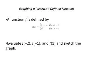

Graphing and Evaluating Piecewise Defined Functions
E N D
Presentation Transcript
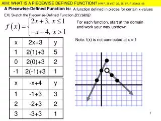
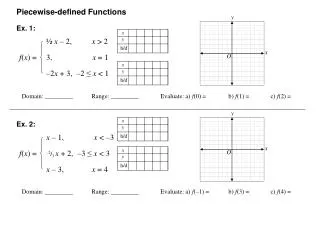
Graphing a Piecewise Defined Function • A function f is defined by • Evaluate f(–2), f(–1), and f(1) and sketch the graph.
Graphing a Piecewise Defined Function • Evaluate f(–2), f(–1), and f(1) and sketch the graph. • Solution: • Remember that a function is a rule. For this particular function the rule is the following: First look at the value of the input x. If it happens that x –1, then the value of f(x) is 1 – x. On the other hand, if x > –1, then the value of f(x) is x2.
Example 9 – Solution cont’d • Since –2 –1, we have f(–2) = 1 – (–2) = 3. • Since –1 –1, we have f(–1) = 1 – (–1) = 2. • Since 1 > –1, we have f(1) = 12 = 1.
Piecewise Defined Functions • How do we draw the graph of f? We observe that if x –1, then f(x) = 1– x, so the part of the graph of f that lies to the left of x = –1 must coincide with the line y = 1 – x, which has slope –1 and y-intercept 1. • If x > –1, then f(x) = x2, so the part of the graph of that lies to the right of the line x = –1 must coincide with the graph of y = x2, which is a parabola.
Piecewise Defined Functions • This enables us to sketch the graph in Figure 17. • The solid dot indicates that the point (–1, 2) is included on the graph; the open dot indicates that the point (–1, 1) is excluded from the graph. Figure 17
Symmetry • If a function f satisfies f(–x) = f(x) for every number x in its domain, then f is called an even function. • For instance, the function f(x) = x2 is even because • f(–x) = (–x)2 = x2 = f(x) • The geometric significance of aneven function is that its graph issymmetric with respect to they-axis (see Figure 19). An even function Figure 19
Symmetry • This means that if we have plotted the graph of f for x0, we obtain the entire graph simply by reflecting this portion about the y-axis. • If fsatisfies f(–x) = –f(x) for every number x in its domain, then f is called an odd function. • For example, the function f(x) = x3 is odd because • f(–x) = (–x)3 = –x3 =–f(x)
Symmetry • The graph of an odd function is symmetric about the origin (see Figure 20). An odd function Figure 20
Example 11 – Testing for Symmetry • Determine whether each of the following functions is even, odd, or neither even nor odd. • (a)f(x) = x5 + x (b)g(x) = 1 – x4(c) h(x) = 2x – x2 • Solution: • (a)f(–x) = (–x)5 + (–x) • = (–1)5x5 + (–x) • =–x5 – x • =–(x5 + x) • = –f(x) • Therefore f is an odd function.
Example 11 – Solution cont’d • (b) g(–x) = 1 – (–x)4 • = 1 – x4 • = g(x) • So g is even. • (c) h(–x) = 2(–x) – (–x)2 • = –2x – x2 • Since h(–x) ≠ h(x) and h(–x) ≠ –h(x), we conclude that h is neither even nor odd.
Symmetry • The graphs of the functions in Example 11 are shown in Figure 21. • Notice that the graph of h is symmetric neither about the y-axis nor about the origin. (c) Neither even nor odd (a) Odd function (b) Even function Figure 21
Example – Combining Two Functions • If and T(v)= 3 – v,find equations and the domains for the functions A(v) = N(v)T(v) andB(v) = N(v)/T(v).
Example – Combining Two Functions • Solution:The formula for the product function is • The domain of is all the real numbers greater than or equal to 0. The domain of T(v)= 3 – v is all real numbers. • The domain of A(v) = N(v) T(v) consists of those values that are shared by both these domains, namely
Example – Solution cont’d Similarly, • Notice that T(v)= 0 when v = 3, so 3 must be excluded from the domain of B. Thus the domain of B is all real numbers greater than or equal to 0, except 3. In set-builder notation, we write
Composition of Functions • There is another way of combining two functions to form a new function. • As a simple illustration, suppose that a company’s annual profit for year t is given by P(t)and the total amount of tax the company pays, f(P), is determined by its profit P. • Since the tax paid is a function of profit and profit is, in turn, a function of t, it follows that the amount of tax paid is ultimately a function of t.
Composition of Functions • In effect, the output of the profit function P can be used as the input for the tax function f, and f(P(t)) is the amount of tax the company paid during year t. • This new function is called the composition of the functions P and f. • The domain of h(x) = f(g(x)) is the set of all values x in the domain of g such that g(x) is in the domain of f.
Composition of Functions • In other words, f(g(x)) is defined whenever both g(x) and f(g(x)) are defined. It is probably easier to picture the composition of f and g with a machine diagram: The h machine is composed of the gmachine (first) and then the f machine.
Example 3 – Composing Two Functions • Let f(x) = x2 and g(x) = x –3. If h(x) = f(g(x)) and k(x) = g(f(x)), compute h(5) and k(5).
Example 3 – Composing Two Functions • Let f(x) = x2 and g(x) = x –3. If h(x) = f(g(x)) and k(x) = g(f(x)), compute h(5) and k(5). • Solution: • First let’s trace the path the input 5 takes under the function h. Since h(5) = f(g(5)), we first input 5 into the inner function g, where g(5) = 2. • The output 2 is then used as an input into the outer function f, which gives an output of f(2) = 22 = 4. • Thus h(5) = f(g(5)) = f(2)= 4.
Example 3 – Solution cont’d Similarly, k(5) = g(f(5)) = g(25) = 22. Notice that the original input always goes through the inner function first, and the resulting output is used as an input into the outer function. We can also write formulas for h and k :
Example 3 – Solution cont’d • Then we can compute • and
Example 4 – Interpreting a Composition of Functions • The altitude of a small airplane t hours after taking off is given by A(t)= –2.8t2 + 6.7t thousand feet, where 0 t 2.The air temperature in the area at an altitude of x thousand feet is f(x) = 68 – 3.5x degrees Fahrenheit. • (a) What does the composition h(t) = f(A(t)) measure? • (b) Compute h(1) and interpret your result in this context. • (c) Find a formula for h(t). • (d) Does A(f(x)) give a meaningful result in this context?
Example 4 – Solution • (a) The hours t that the airplane has been flying is first used as an input into the inner function A, which outputs the altitude of the plane A(t) in thousands of feet. • This altitude in turn is used as an input into the outer function f, which outputs a temperature in degrees Fahrenheit. • Thus h is the air temperature at the airplane’s location t hours after take-off.
Example 4 – Solution cont’d • (b) The input 1 first enters the function A, giving A(1)= 3.9. • We then input 3.9 into the function f, which gives f(3.9)= 54.35. • This means that 1 hour after take-off, theair temperature at the plane’s location is 54.35F.
Example 4 – Solution cont’d • (c) h(t) = f(A(t)) = f(–2.8t2 + 6.7t ) • = 68 – 3.5 (–2.8t2 + 6.7t ) • = 9.8t2 – 23.45t + 68 • Using this direct formula, you can verify that h(1) = 54.35 as we found in part (b).
Example 4 – Solution cont’d • (d) Although we could compute a formula for A(f(x)), it wouldn’t be a meaningful quantity here. • The inner function f outputs a temperature in F, but this is not an appropriate value to pass to the outer function A as an input, because A is a function of t, a number ofhours.
Composition of Functions • So far we have used composition to build complicated functions from simpler ones. • But we will see in later chapters that in calculus, it is often useful to be able to decompose a complicated function into simpler ones, as in the next example.
Example 5 – Decomposing a Function • If L(t)=(2t – 1)3, find functions f and g such that L(t)= f(g(t)).
Example 5 – Decomposing a Function • If L(t)=(2t – 1)3, find functions f and g such thatL(t)= f(g(t)). • Solution: • The formula for L says: First double t and subtract 1, then cube the result. One option is to think of 2t – 1 as the inner function and call it g. • Then g(t)=2t – 1 and L(t)=(g(t))3. The outer function is the cubing function, so if we let f(x)= x3, then
Example 5 – Solution cont’d • Note that there are other choices we could have made, such as g(t)=2t and f(x)=(x –1)3, but the first solution is probably the most useful one.
Linear Models and Rates of Change Of the many different types of functions that can be used to model relationships observed in the real world, one of the most common is the linear function. When we say that one quantity is a linear function of another, we mean that the graph of the function is a line.
Review of Lines The slope of a line is a measure of its steepness. We measure the slope by computing the “rise over run” between any two points on the line: As we can see above, the rise is simply the difference or change in y-values between the two points and the run is the difference in x-values.
Review of Lines Thus we can think of the slope as the “change in y over the change in x.”Now let’s find an equation of the line that passes through a given point (x1, y1) and has slope m.
Review of Lines If we compute the slope from (x1, y1) to any other point(x, y) on the line, we get which can be written in the form y – y1 = m(x – x1) This equation is satisfied by all points on the line, including (x1, y1), and only by points on the line.
Review of Lines Therefore it is an equation of the given line. Equation 2 becomes even simpler if we use the point at which a (nonvertical) line intersects the y-axis.
Review of Lines The x-coordinate there is 0 and the y-value, called the y-intercept, is traditionally denoted by b.
Review of Lines Thus the line passes through the point (0, b) and Equation 2 becomesy – b = m(x – 0)which simplifies to the following:
Example 1 – A Line through Two Points Find an equation of the line through the points (–1, 2) and (3, –4) and write the equation in slope-intercept form. Solution: By Definition 1 the slope of the line is Using Equation 2 with x1 = –1 and y1 = 2, we obtain
Example 1 – Solution cont’d which can be written as or
Rate of Change and Linear Functions The slope of a line is the ratio of the change in y, y, to the change in x, x. Thus we can interpret the slope as the rate of change of y with respect to x. If f is a linear function, then its graph is a line and we can think of the slope as the ratio of the change in output to the change in input. In this context, the slope measures the rate of change of the function.
Rate of Change and Linear Functions The slope of a given line is the same at all points, so a characteristic feature of linear functions is that the rate of change is constant: Linear functions grow at a constant rate. A rate of change is always measured by a ratio of units: output units per input unit.
Example 3 – Slope of a Linear Function A company that produces snowboards has seen its annual sales increase linearly. In 2005, it sold 31,300 snowboards, and it sold 38,200 snowboards in 2011. Compute the slope of the linear function that gives annual sales as a function of the year. What does the slope represent in this context? Solution:The slope is
Example 3 – Solution So the slope is 1150, and the units are number of snowboards per year. Thus the number of snowboards the company produces is increasing at a rate of 1150 per year. cont’d
Rate of Change and Linear Functions Because the graph of a linear function is a line, we can write an equation for a linear function using the slope-intercept form f(x)= mx+b
Example 6 – Writing a Linear Model Using the Point-Slope Form A pump has been pouring water into a swimming pool. The data in the table show the water volume of the pool every two hours after the pump was activated. (a) Explain why a linear model is appropriate. (b) Write an equation for a linear function to model the data.(c) Use your model to predict the volume of water in the pool after 17.5 hours.
Example 6 – Writing a Linear Model Using the Point-Slope Form (d) When will the amount of water in the pool reach 6000 gallons? Solution: (a) The volume of water increases 300 gallons during each two-hour interval. Thus the rate of change is constant, indicating a linear relationship between the input and output. (b) The rate of change is 300 gallons every two hours, or 150 gallons per hour, so the slope is m = 150.
Example 6 – Solution If we let V(t)be the water volume in gallons t hours after the pump is activated, then V(2) = 2800, so the point (2,2800) is on the graph. The point-slope formula givesV – 2800 = 150(t – 2) = 150t – 300 V = 150t + 2500 Thus the water volume in gallons t hours after the pump is turned on is given by V(t) = 150t + 2500. cont’d
Example 6 – Solution (c) The volume of water in the pool after 17.5 hours is V(17.5) = 150(17.5) + 2500 = 5125 gallons. (d) We solve V(t) = 6000: 150t + 2500 = 6000 150t = 3500 cont’d
Example 6 – Solution Thus the amount of water in the pool reaches 6000 gallons after hours, or 23 hours 20 minutes. cont’d