Numbers, Measurement, and Uncertainty for Physics and MOSAIC

1. Numbers, Measurement, and Uncertainty for Physics and MOSAIC A Physics MOSAIC MIT Haystack Observatory RET Revised 2011 Background Image by SKMay

2. Numbers in Science vs. Numbers in Mathematics This lesson is designed to help provide some intuition for the way numbers are used in science. This can often be different from the way you are used to thinking about numbers in mathematics. For example, while every digit that comes out of your calculator is often important in mathematics, it is almost never a good idea to include every digit that comes from your calculator in an answer for science class.

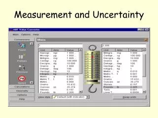
3. Making a Measurement The key to understanding numbers in science is an understanding of measurement. There is a fundamental difference between numbers as a mathematical concept that we use for counting or calculation and the numbers we derive from measurements of the physical world. The reason for this is that no measurement is exact. There is always some inherent estimation involved in making a measurement. Photo from Wikipedia user André Karwath aka Aka, Creative Commons Photo by SKMay Photo from Wikipedia user MJCdetroit, Creative Commons

4. Reporting a Measurement • To be truly scientific, every measurement should include both the value and uncertainty associated with it. That is, measurement = best estimate ± uncertainty. The uncertainty is a measure of the confidence in the estimate. • For example, on the previous slide, we might record • 199 ± 1 mL 21.0 ± 0.1 mm 0.385 ± 0.0005 V • Because we encounter numbers all the time that are not in this format and instead include only the measurement, we should agree on a convention: • The number of digits reported in any measurement should follow the rule, agreed upon by all scientists: exactly one estimated digit is significant, and therefore, exactly one estimated digit is reported. • While it is preferable to record actual uncertainties in your measurements, the implicit rule is that your uncertainty is ± position of last record digit. • Therefore, a mass of 68.5 kg is implicitly 68.5 ± 0.1 kg.

5. Significant Figures Because scientists have agreed on a convention that exactly one estimated digit is significant, one can assume that the smallest recorded digit corresponds to the estimate. Consider the following examples:

6. Sources of Uncertainty • What does the uncertainty depend on? • The resolution (or exactness, or precision) of your measuring device. • You can’t be sure of more digits than your device reports. • Usually, you can estimate one extra digit beyond what is marked by estimating where the measurement lies between the two marked values. • For digital meters, it’s not always clear where the uncertain digit is, but, unless it is clear that the digits reported are not certain (because they are changing, for example), it can be assumed to be one digit beyond what is recorded. • The care with which you collect your data, and the nature of what you are measuring. • There are times when a measuring device provides more resolution (or precision, or exactness) than is necessary or possible to take advantage of. • For example, when measuring the height of a friend using a meter stick, you probably are not certain of the distance down the millimeter, even though they are marked on the device. Your friend’s head is probably a little fuzzy and irregular. • It is better to communicate honestly your uncertainty than to include extra digits that imply greater precision than was observed. For example, h = 165 ± 0.5 cm, or maybe even 165 ± 1 cm.

7. Error Bars Error bars are not commonly used in high school science courses, but they are a useful way of picturing the uncertainty associated with a measurement. Consider the following measurements of volume and mass as the baby bottle from a previous slide is consumed. Implicit in each measurement of volume is an uncertainty of ± 1 mL, and implicit in each measurement of mass is an uncertainty of ± 10 g. How can we communicate that in a graph of this data?

8. Interpreting Data from Other Scientists Whenever you hear or read a statistic or fact derived from scientific measurement, you should consider the associated uncertainty. Remember, no measurements are exact, and a good scientist (or journalist) will include some indication of uncertainty associated with the number being reported. Most scientific data included in scientific papers will include actual uncertainties, in either absolute or percentage form. Many resources for the general public (and even, many times, those for scientists!) will not include any explicit uncertainty, and may even intentionally report the findings with fewer significant figures than were observed. Excerpt from Physical Review Focus (focus.aps.org), The Americal Physical Society, 2 July 2010, The Coolest Anti-Protons, used with permission

9. Interpreting Data, Again This article about a recently discovered planet orbiting a “nearby” star identifies the distance to the star as 40 light years. What is the implied uncertainty in this value? Does this accurately reflect the actual uncertainty in the scientific community in this value? Article from MIT News, Image by Jason Rowe, NASA/Ames; Jaymie Matthews, UBC, used with permission

10. More About Uncertainty Sometimes, the implied uncertainty is misleading, and the actual uncertainty is either a less or more than indicated by the reported digits. Example 1: 400 m Track Example 2: Food Labels; 25 g carbohydrate Photo by thetorpedodog, found on Flickr, Creative Commons Photo by SKMay

11. Measurement Error: Random • There are a number of good reasons your measurement might not be exactly the same as someone else’s. For example… • You might apply more or less pressure to the end of the caliper, causing small deformations in the size of the material being measured. • You could be slightly above or below water level when reading the volume of liquid in the bottle. • Small variations in temperature might have affected the resistance of the multimeter, thereby changing slightly the voltage recorded. • These errors are collectively referred to as random (or statistical) errors. This is a graphical depiction of random error. Note that instead of a single data point, the “true value” in this case is a distribution, as will be in the MOSAIC system. http://metazoaludens.wikidot.com/elvin-18-may, Creative Commons

12. Measurement Error: Systematic • There are other reasons your measurement might not be the same as the true value . For example… • The bottle could contain a solid item, thus displacing fluid and leading to volume measurements that are bigger than the true value. • The calipers could be offset from the true diameter of the ball, resulting in a reading that is smaller than the true value. • The voltmeter could be reading an additional voltage source along with the one of interest, resulting in a reading either higher or lower than the true value. • These errors are collectively referred to as systematic errors. http://metazoaludens.wikidot.com/elvin-18-may, Creative Commons

13. Summary:Random vs. Systematic Error Random errors are unavoidable. They will be present to some extent no matter how careful the experimenter is. The question, then, is how to determine whether or not systematic error is present. Consider the effect of each of type of error on the following quantities as the number of measurements is increased.

14. Another Possibility? When conducting experiments in science class, you should also keep in mind that even when you “know” the “answer” (or accepted value) for a measurement or calculation, there is always uncertainty associated that value, as well. A good rule of thumb is that if your uncertainty includes the accepted value OR if the accepted value’s uncertainty includes your measurement, the two are consistent. Example 1: The acceleration due to gravity has an accepted value of 9.81 (± 0.01) m/s2. You conduct an experiment and find the acceleration due to gravity is 9.9 ± 0.1 m/s. Is your value consistent with the accepted value? Example 2: A lens included as part of an introductory optics kit is labeled with a focal length of 150 mm. You conduct a careful experiment to verify this fact, and determine the focal length to be 142 (± 1) mm. What is the assumed uncertainty on the given focal length? Is your value consistent with the labeled value? Example 3: Galaxy Z has a published magnitude of 8.8 in the astronomical tables, but one night, you make an observation of it and find its magnitude to be 5.73 ± 0.01. Is this consistent with the published value? What could account for the discrepancy?

15. Data Sets When many measurements are made of the same physical system, one can create a data set. Recall that each individual measurement will be affected by random error and may be affected by systematic error, but one can think of the set as a whole as being characterized by properties such as its mean, accuracy, precision, standard deviation, and standard error of the mean. The first three of these are probably familiar to you. In words, Mean: Average measurement Mode: Most common measurement Median: Middle measurement (halfway between highest and lowest) Accuracy: measure of how close measurements are to true value Precision: measure of how close measurements are to each other. Images from Wikipedia, Public Domain

16. When to Average • A few rules of thumb on when it makes sense to average your measurements: • When you have measured the same quantity the same way at (nearly) the same time. • Example: Multiple measurements of the height of your friend. • When you have measured the same quantity in the same (or very similar) way at different times that don’t make any difference to the value. • Example: Multiple measurements of a ball being dropped from a table. • When you have measured the same (or very similar) quantity in the same (or very similar) way at different times that might make a difference to the value, but not one you are interested in. • Example: Multiple measurements of daily growth of a plant throughout the summer. • Example: Height measurements of multiple students • NOTE: It is not a good idea to average when you are attempting to observing a trend in the data. That is, if you expect the data will not provide the same value, don’t average.

17. Distributions and Histograms A set of data is often called a distribution due to the variety of values observed. Often, these distributions are plotted as a histogram, plotting the values along the x-axis and the number of occurrences of each value on the y-axis. Consider the following list of semester grades for Physics 11. The histogram for this data is shown.

18. Normal Distribution A normal distribution is one where a histogram of the data assumes a bell-shaped (or Gaussian) shape. The distribution is symmetric. The mean, mode, and median are the same in such a distribution. Galton Box, from Wikipedia, Antoine Taveneaux, Creative Commons

19. Normal Distribution:Graphical Depiction of Errors If we consider a normal distribution of data, we can graphically interpret the precision and accuracy of the data without need to reference the bulls eye diagrams from before. In such a plot, the accuracy and precision can be characterized as shown below. Image from Wikipedia, user Pekaje, GNU Documentation

20. Large Data Sets:Standard Deviation The standard deviation within in a set of data provides a measure of how close together the data points are. If the data follow a normal distribution, we would expect 68.2% of all data points to be within one standard deviation of the mean, 95% of all data points to be within 2 standard deviations of the mean, and 99.7% of all data points to be within 3 standard deviations of the mean. Standard deviation diagram, based an original graph by Jeremy Kemp, in 2005-02-09 [http://pbeirne.com/Programming/gaussian.ps]. From Wikipedia, Creative Commons.

21. Standard Deviation Math The standard deviation (s) is, in words, the square root of the average for all measurements of the square of the difference that measurement and the average. Symbolically, Where

22. Standard Deviation Example Example: For the semester grades seen on an earlier slide, we can compute the standard deviation. Now we need to add those up, divide by 16 (the total number), and take the square root.

23. Large Data Sets:MOSAIC Data Consider a large data set consisting of a single measurement that is not affected by systematic error. The standard deviation associated with the random error depends on the instrument being used and experimental technique. It will not change as more trials are conducted. What will happen, however, is that the mean of the measurements will become closer and closer to the true value as more measurements are made. The distribution will more closely resemble a normal distribution as the number of trials is increased. ! ?

24. Quantifying the Advantage of “Large” • As we saw, the standard deviation is somewhat inherent to the system making the measurement. Our confidence in the average value, however, increases with an increase in sample size. This can be expressed with a quantity called standard error of the mean (SEM). • When working with large sets of data, this is the quantity that is most often used to place error bars on each data point. • Note that: • The SEM increases as the standard deviation increases. (This should make sense; the greater the standard deviation, the less sure you will be of your average.) • The greater the number of trials, the smaller the SEM. (This should make sense; with more trials comes more confidence that the average of your data set is the true value.) • Because the SEM decreases only with the square root of the number of trials, it becomes very difficult (and expensive) to reduce the SEM by increasing the number of trials. For a decrease of a factor of 2, the number of trials must increase by _____ (?).

25. Placing Error Bars: MOSAIC data This plot shows the relationship between mesospheric ozone for the first 4 days of 2010. The data is averaged into 30 minute bundles and consists of data from 5 different sites averaged together. The error bars reflect the standard error of the mean. The circled data point comes from 15 ten minute different observations of mesospheric ozone. This plot shows the relationship between mesospheric ozone for the first 1 day of 2010. The data is reported every 10 minutes and consists of data from only one site. The error bars reflect the standard error of the mean. The circled data point comes from 1 ten minute observation of mesospheric ozone.

26. Spectral View While both spectra clearly include a lot of noise, the spectrum on the left (corresponding to 5 sites averaged over four days) is clearly more discernible above the noise than that on the right (corresponding to 1 site averaged over one day).