Coase Theorem
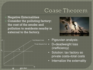
Private Marginal Cost. Coase Theorem. Pigouvian analysis: D=deadweight loss (inefficiency) Solution: tax factory so private costs=total costs Internalize the externality. P. Total Marginal Costs. D. P m. Negative Externalities

Coase Theorem
E N D
Presentation Transcript
Private Marginal Cost Coase Theorem • Pigouvian analysis: • D=deadweight loss (inefficiency) • Solution: tax factory so private costs=total costs • Internalize the externality P Total Marginal Costs D Pm Negative Externalities Consider the polluting factory: the cost of the smoke and pollution to residents nearby is external to the factory. Q Q* QToo Much
P Total Marginal Costs Private Marginal Cost D A C B Q Q* QToo Much Coase Theorem • Cutting back means the firms loses C in producer surplus. • Nearby homeowners benefit by D+C, more than the losses to the factory. • If transaction costs are low the two parties should be able to find an exchange to make both better off. • e.g. homeowners pay factory D/2+C to reduce output to Q* • Both parties gain! In 1960 Coase showed that the Pigouvian analysis was wrong. External costs do not necessarily create inefficiencies. Consider our polluting factory. If firm cuts output from QToo Much to Q* it loses how much?
Coase Theorem Private marginal costs when transaction costs are low and damages tax is imposed Private marginal costs when transaction costs are low P Private Marginal Cost, traditional view • Now look at effect of damages tax • An efficient outcome becomes an inefficient one! D A C B • Market will internalize some externalities automatically • Opportunity cost • If homeowners are willing to pay to have externality reduced then the external cost is a cost to the firm. • A profit maximizing firm will take into account the costs it imposes on others as long as it is efficient to do so Q QToo Little Q* QToo Much
Divorce in the U.S. The divorce rate in the United States has increased significantly over last 30 years. One way to classify divorce: unilateral vs. mutual. Under a mutual divorce rule both parties must agree to divorce. Under a unilateral divorce rule only one party needs to desire divorce for the divorce to be granted. In the 1970s there was a movement towards unilateral divorce.
Coase and Divorce • Using the assumptions and predictions of the Coase theorem what should be effect of either law on divorces? • Consider John and Mary and Tom and Gerri, who place different values on being married: • Coase theorem says that John and Mary should stay together, and Tom and Gerri should split up. • Unilateral divorce: John pays Mary to stay together; Tom and Gerri divorce with no payment. • Mutual divorce: Tom pays Gerri to divorce; John and Mary stay together with no payment. Image from Divorce-Education.com
Coase and Divorce • Law should not change the number of divorces, divorce still takes place when joint benefit of marriage < joint cost of marriage • It should, however, effect how partners are compensated • Mutual divorce gives “property rights” to the spouse that wants to stay married, they must be compensated in order for a divorce to ocurr. • Unilateral divorce gives “property rights” to the spouse who wants to leave, they must be compensated if the marriage is to stay intact.
Coase and Divorce The actual effect of the change in trend from mutual to unilateral divorce on divorces in the United States has been debated in the literature. Elizabeth Peters (1986) finds that this change had no effect on the number of divorces, but did effect compensation in the form of spousal support at divorce. Leora Friedberg (1998) finds the shift to unilateral divorce had a positive and permanent effect on the divorce rate (but explains only 17 percent of the change in divorce rates between 1968 and 1988.) Justin Wolfers (2006) argues that this positive effect was only temporary, and leveled off after about a decade so that in the end it had no discernable effect. Stevenson/Wolfers (2003) show the effect of divorce law change on well-being and spousal relations.
Peters (1986) • Peters suggests two possible models for the marriage contract • Symmetric Information • Both spouses have the same information about the value of their alternatives to marriage (value of divorce) • Bargaining is costless • Similar to Coase theorem assumptions • Asymmetric Information • Neither spouse knows the value of the other’s alternatives • Incentives to lie about opportunities to gain larger share of marital wealth • Bargaining is successfully prevented
X=Initial marriage wage for wife • Aw/h=Value of opportunities outside of marriage for wife or husband • Wife wants divorce when Aw>X (A,C,D) • M is the joint product in marriage. • Husband when Ah>M-X or M-Ah<X (A,E,F) • They agree in A, but disagree elsewhere.
With symmetric information a compensation scheme exists so that divorce will only occur when JOINT benefit < JOINT cost (Areas A, C, E) • However, if bargaining is prevented by asymmetric information: • Under mutual rule then divorce will only occur in A, where both parties agree (lower than optimal) • Under unilateral rule divorce will occur in all highlighted areas (A + C + E + F + D) when either spouse desires divorce (higher than optimal) Result: Under symmetric information law should not change number of divorces Under asymmetric information we get more divorces under unilateral rule than mutual rule
Empirical Test • Data on individuals from the March/April 1979 Current Population Survey • Demographic Variables (age, children, income, education, etc..) • For those ever divorced: marital history, spousal support, value of property settlements • Categorized state divorce laws three ways • Pure unilateral • Mutual divorce (with binding arbitration if no agreement) • Unilateral divorce possible, but large cost involved (i.e. separation periods). Due to burden of high cost these states are included under mutual divorce • Note from Table 3 the sample sizes!
Empirical Test • Logit regression • Dependent variable: Probability of becoming a divorcee during 1975-1978 given no previous divorces • Controls: • Demographic variables • Region of the US the woman lives • State Divorce Rate in 1970 • Used to control for any unobserved propensity for divorce in the given state • Percent of Catholics in the state of residence • Unilateral: a dummy variable, =1 if state of residence has pure unilateral laws, =0 otherwise.
The probability of divorce decreases with age, education, kids under 18 and varies somewhat by region. • Most importantly the coefficient on unilateral is not statistically significant and negative (!) in one regression. • Remarriage is less likely in a state with unilateral divorce. Why? • But remember the sample size! • If such an effect exists is it consistent with Coase? Peters, H. Elizabeth. Marriage and Divorce: Informational Constraints and Private Contracting
Compensation • Under unilateral divorce there is compensation to keep the marriage together – compensation goes to the party that wants out of the marriage. • Under mutual divorce there is compensation to get the divorce – compensation goes to the party that wants to stay in. • Therefore at divorce we should expect to see more compensation under mutual divorce then under unilateral. • Divorce settlements consist of: • Alimony • Child Support • Property Settlement • We should also see a higher variance of settlement payments under mutual divorce since you have to compensate the worse off spouse which could be the husband or wife, while compensation payments are not required under unilateral divorce.
Peters, H. Elizabeth. Marriage and Divorce: Informational Constraints and Private Contracting
Variance of settlements are larger in mutual states. • Mean is also lower in unilateral states, however, so we may want to look at variance relative to the mean. • Thus Peters look also at the “coefficient of variation.” What is this? • In both cases the compensation is more variable in mutual states although less so for the coefficient of variation than the pure variance. Peters, H. Elizabeth. Marriage and Divorce: Informational Constraints and Private Contracting
Peters’ Conclusion • Empirical results point to symmetric information model (Coase theorem model) • Bargaining occurs such that divorce only takes place when joint benefit < joint cost, law has no effect on number of divorces • Law does have effect on compensation schemes • Alimony/Child Support are lower in unilateral states • Variance of payments is higher in mutual divorce states
Friedberg (1998) • Assumes same model as used in Peters (1986) • Attempts to reconcile Peters (1986) and Allen (1992) • Allen(1992) argued that region dummies and state divorce rate in 1970 just absorb the variation in divorce laws and should not be included. He found a significant, positive effect of unilateral divorce laws on divorce rates.
Friedberg’s (1998) response/Empirical Test • Claims there are two major difficulties in literature • Controlling for differences in state/regional divorce propensities • Defining and categorizing state divorce laws • Uses state level divorce rates as dependent variable rather than individual propensities to divorce. • Uses state fixed effects: serve same purpose as Peters inclusion of 1970 divorce rate but is more general. • Adds state-specific time-trends to model • allows unobserved state divorce propensities to trend linearly or quadratically and vary across states • Model: • Divratest = c0 + c1*unilateralst + c2s*states + c3s*yeari + c4s*states*timet + c5s*state*timet2 + ust • Data on state divorce rates from Vital Statistics of the United States.
Regression 3.3 is similar to Peters’ with state fixed effects (Peters included state’s 1970 divorce rate). Note that without fixed effects the result is positive and with fixed effects the affect disappears. What does this mean? What does it imply about the unobserved variable? • 3.4 and 3.5 then introduce linear and quadratic state trends. Note that there are still year effects in the regression so what do these mean?
Friedberg(1998) • Unilateral raised the divorce rate. • Thus only impefect Coasian bargaining takes place among spouses. • State-specific trends matter. • Note, however, that her estimate is that unilateral raised the divorce rate by about 10% or .4/4.6 per thousand. The divorce rate doubled between about 1960 and 1980 from around 2.2 to 5 so unilateral explains perhaps 14-15% of the increase. Much less than one might imagine. A picture tells the real story.
Friedberg (1998) • Besides the endogeneity issue, another issue plaguing research on divorce laws is classification of states as unilateral or mutual • Some unilateral states impose a mandatory separation period which may impose a high cost on unilateral divorce • Other no-fault unilateral states still have fault grounds for property settlement, which could distort property rights from the spouse wishing to leave to the one wishing to stay • Friedberg classifies “very strict” unilateral divorce as divorce with no separation requirement and no fault grounds for property settlement.
Type of unilateral divorce matters • Versions of unilateral divorce that impose more requirements have smaller effects, i.e. strictest form of unilateral divorce raises divorce rates the most.
Endogoneity • Did rising divorce rates cause a state to change its law from mutual to unilateral? If so, the effect of unilateral on divorce rates will be confounded by reverse causality. • Best solution is instrumental variables. Find a variable correlated with the change in the law but not with divorce rates. • E.g. # of women in the state legislature? • # of state legislators who have been divorced? • Whether a state has a referendum possibility? • Friedberg doesn’t use IV but she does make an interesting observation: • She finds that the divorce rate does predict if a state adopts a unilateral law but not when it adopts such a law. Since she has fixed effects in her regression the estimated effect is identified by what happens within a state when the law changes and not by differences across the states – hence she suggests she is ok on this issue. • But there is something peculiar going on. (Recall our discussion of fixed effects and omitted variables.) Without state trends the effect of unilateral is zero and with trends it is positive so the omitted variable which is correlated with unilateral must be negatively correlated with trends in divorce rates, ie. Driving divorce rates down. But the most plausible argument is that states that passed unilateral laws did so because of omitted variables that would have driven the divorce rate up!
Friedberg(1996) - Conclusions The method of controlling for geographical heterogeneity in divorce propensities is important More flexible controls of unobserved characteristics is crucial Significant, positive, permanent impact of the switch to unilateral divorce law on divorce rates
Problems • Are state fixed effects/trends always a good idea? • The problem of efficiency • The problem of dynamic effects
Wolfers (2006) Again assumes similar model as in Peters (1986) Concerns about sensitivity to state-specific trends in Friedberg’s model Besides endogeneity issue, a major problem is separating pre-existing trends from dynamic effects of a policy shock Thus, Wolfers considers that divorce can have a dynamic response to changes in the law (policy shock) Believes that immediately following reform there could be a large rise in the divorce rate due to pent-up demand for unilateral divorce
Vertical line at 1969 represents change from mutual to unilateral divorce • The bold line represents Wolfers hypothetical model, where divorce spikes right after law change, then eventually levels off to new steady state. • Notice Friedberg’s trend is derived mostly from post-change data. • Lines marked “Before” and “After” represent the average difference between the divorce rate and trend before and after legal change • This difference is what is picked up in the “unilateral” dummy variable in Friedberg’s regression • Compare before and after after subtracting post-law trend with true difference. • Thus Friedberg’s model may overstate effect of law change in the long run
Wolfers(2006) Empirical Test • Adds dummy variables that model the dynamic response: • For first two years of new legal regime • Then years three, four, five, etc.. • Dependent variable is divorce rate • Includes state fixed effects, time fixed effects, and state-time effects
All three regressions suggest that divorces spiked immediately after legal change, and then the effect declines over subsequent years
Wolfers(2006) • Also does analysis on the stock of divorces. • Finds, following Gruber, that the stock of divorces increases (contrary to the earlier results). • But currently divorced population from census data does not include those that have remarried • Data show that only 49% of those ever-divorced are currently divorced • So Wolfers creates a measure of the ever-divorced population: which includes those currently divorced and those currently married, separated, or widowed but are on their second marriage • Then analyzes effect of divorce law on ever-divorced population
No effect of divorce laws on ever-divorced population by 1980
Wolfers(2006) Though there is an immediate spike in divorce rate following the switch to unilateral divorce, this effect falls over time In the long run the switch to unilateral divorce appears to have no discernible effect on the amount of divorces or the size of the ever divorce population Both regressions seem to indicate that unilateral divorce laws explain only a small fraction of large rises in divorce rates
Divorce and Coase Coasian prediction is much closer to reality than the opposite. Let p=prob. that divorce will be desired. Then p^2 is prob. both partners will desire divorce. Assume a mutual consent state and no bargaining then p^2 is the divorce probability. Divorce in states with unilateral divorce should then be 2p-p^2 In mutual consent state in 1960 about .2 are divorced thus .2=p^2 and p=.45 so increase in divorce should be on the order of 2p-p^2-p^2=.9-.2-.2=.5=50%! Actual increase is 0.5% Thus Coasian bargaining very much supported.
Divorce Laws and Family DistressStevenson and Wolfers (2003) • Coase Theorem says no impact of divorce law on number of divorces. Coase Theorem holds up well empirically. • But Coase Theorem also says that changing from mutual to unilateral divorce changes the bargaining power of spouses. • This effects spousal relations and well-being even if it has no effect on the divorce rate. • Recall: • Mutual divorce gives “property rights” to the spouse that wants to stay married, they must be compensated in order for a divorce to occur. • Unilateral divorce gives “property rights” to the spouse who wants to leave, they must be compensated if the marriage is to stay intact. • Women file for divorce more often than men so there is a suggestion that unilateral divorce benefits women.
There is no necessary benefit to women, however. • Three measures of well-being and spousal relations: suicide, domestic violence and spousal murder. • Expected sign is difficult to hypothesize: • Suicide and Divorce may be substitutes, so easier divorce could mean a lower suicide rate. • Easier divorce may leave more upset and abandoned spouses, increasing suicide rate. • Unilateral divorce offers a credible threat of exit which may reduce domestic violence. • However, domestic violence could be used to enforce the marriage contract which the law no longer offers.
Models of Intra-Family Bargaining Common preferences – Rotten Kid Theorem. Threat Points – internal and exit.
Empirical Analysis Use state-based panel data A dummy variable indicates whether the state had unilateral divorce at that time State and time fixed effects are included in all regressions Dependent variables: suicide rate, domestic violence (a dummy variable indicating whether a specified type of violence occurred in the household), intimate murder rate.
Suicide • Dependent variable: suicide of all persons • Controls: • unilateralk, a series of dummies that equal one if a state changed to unilateral divorce k years ago (thus shows dynamic response of the suicide rate • State fixed effects • Year fixed effects • Male/Female employment rates, state income per capita, unemployment, share of state population on welfare, availabilty of abortion, racial/age composition of state • Also disaggregated data on women by age • Would expect smaller or no effect in very young and very old women
Statistically significant reduction in female suicides after change to unilateral regime • No effect on male suicide • Adding controls hardly changes effect of unilateral divorce • Note, however, that with state specific time trends less can be concluded.
Note that there is little or no evidence that suicide leads the change in divorce law.
Little or no effect of switch to unilateral divorce on teens and the elderly
Domestic Violence Data comes from Family Violence Surveys in 1976 and 1985 Compares treatment states (those who changed to unilateral divorce) to control states (those yet to adopt unilateral or those with pre-existing regimes involving unilateral divorce) Expect changing violence propensities in treatment group relative to controls
Treatment led to a decrease in husband to wife domestic violence rates. • Note that a large fraction of the change comes from the control states.