Download
1 / 40
400 likes | 548 Views
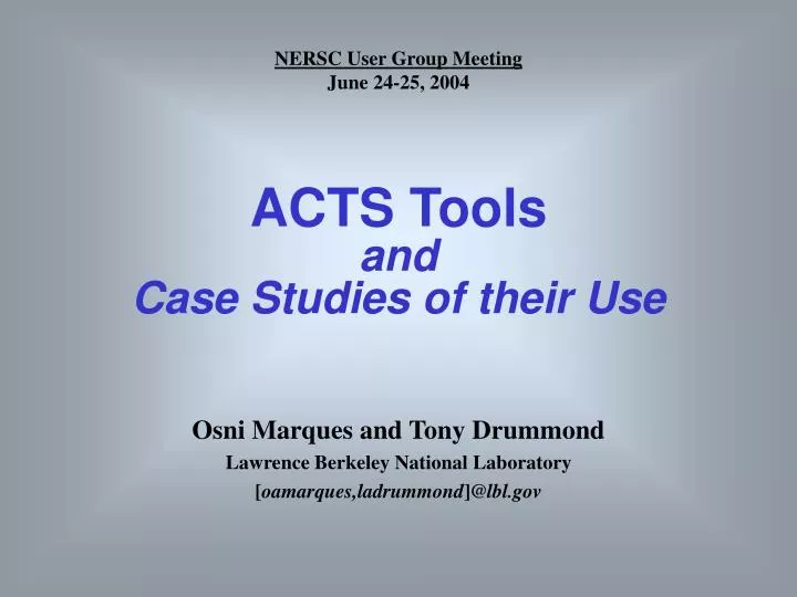
NERSC User Group Meeting June 24-25, 2004. ACTS Tools and Case Studies of their Use. Osni Marques and Tony Drummond Lawrence Berkeley National Laboratory [ oamarques,ladrummond ] @lbl.gov. What is the DOE ACTS Collection?. High Intermediate level Tool expertise Conduct tutorials.

E N D
NERSC User Group Meeting June 24-25, 2004 ACTS Toolsand Case Studies of their Use Osni Marques and Tony Drummond Lawrence Berkeley National Laboratory [oamarques,ladrummond]@lbl.gov
What is the DOE ACTS Collection? • High • Intermediate level • Tool expertise • Conduct tutorials • Advanced CompuTational Software Collection • Tools for developing parallel applications • ACTS started as an “umbrella” project • Intermediate • Basic level • Higher level of support to users of the tool • Basic • Help with installation • Basic knowledge of the tools • Compilation of user’s reports Goals • Extended support for experimental software • Make ACTS tools available on DOE computers • Provide technical support • Maintain ACTS information center • Coordinate efforts with other supercomputing centers • Enable large scale scientific applications • Educate and train http://acts.nersc.gov acts-support@nersc.gov NERSC User Group Meeting
Motivation 1: Challenges in the Development of Scientific Codes • Libraries written in different languages. • Discussions about standardizing interfaces are often sidetracked into implementation issues. • Difficulties managing multiple libraries developed by third-parties. • Need to use more than one language in one application. • The code is long-lived and different pieces evolve at different rates • Swapping competing implementations of the same idea and testing without modifying the code • Need to compose an application with some other(s) that were not originally designed to be combined • Productivity • Time to the first solution (prototype) • Time to solution (production) • Other requirements • Complexity • Increasingly sophisticated models • Model coupling • Interdisciplinarity • Performance • Increasingly complex algorithms • Increasingly complex architectures • Increasingly demanding applications NERSC User Group Meeting
Motivation 2: Addressing the Performance Gap through Software 1,000 Peak Performance 100 Performance Gap 10 Teraflops 1 Real Performance 0.1 1996 2000 2004 Peak performance is skyrocketing • In 1990s, peak performance increased 100x; in 2000s, it will increase 1000x But • Efficiency for many science applications declined from 40-50% on the vector supercomputers of 1990s to as little as 5-10% on parallel supercomputers of today • Need research on • Mathematical methods and algorithms that achieve high performance on a single processor and scale to thousands of processors • More efficient programming models for massively parallel supercomputers NERSC User Group Meeting
ACTS Tools Functionalities NERSC User Group Meeting
Use of ACTS Tools Model of a "hard" sphere included in a "soft" material, 26 million d.o.f. Unstructured meshes in solid mechanics using Prometheus and PETSc (Adams and Demmel). 3D incompressible Euler,tetrahedral grid, up to 11 million unknowns, based on a legacy NASA code, FUN3d (W. K. Anderson), fully implicit steady-state, parallelized with PETSc (courtesy of Kaushik and Keyes). Multiphase flow using PETSc, 4 million cell blocks, 32 million DOF, over 10.6 Gflops on an IBM SP (128 nodes), entire simulation runs in less than 30 minutes (Pope, Gropp, Morgan, Seperhrnoori, Smith and Wheeler). Molecular dynamics and thermal flow simulation using codes based on Global Arrays. GA have been employed in large simulation codes such as NWChem, GAMESS-UK, Columbus, Molpro, Molcas, MWPhys/Grid, etc. Electronic structure optimization performed with TAO, (UO2)3(CO3)6 (courtesy of deJong). 3D overlapping grid for a submarine produced with Overture’s module ogen. NERSC User Group Meeting
Use of ACTS Tools Two ScaLAPACK routines, PZGETRF and PZGETRS, are used for solution of linear systems in the spectral algorithms based AORSA code (Batchelor et al.), which is intended for the study of electromagnetic wave-plasma interactions. The code reaches 68% of peak performance on 1936 processors of an IBM SP. Induced current (white arrows) and charge density (colored plane and gray surface) in crystallized glycine due to an external field (Louie, Yoon, Pfrommer and Canning), eigenvalue problems solved with ScaLAPACK. Omega3P is a parallel distributed-memory code intended for the modeling and analysis of accelerator cavities, which requires the solution of generalized eigenvalue problems.A parallel exact shift-invert eigensolver based on PARPACK and SuperLUhas allowed for the solution of a problem of order 7.5 million with 304 million nonzeros. Finding 10 eigenvalues requires about 2.5 hours on 24 processors of an IBM SP. OPT++is used in protein energy minimization problems (shown here is protein T162 from CASP5, courtesy of Meza , Oliva et al.) NERSC User Group Meeting
PETSc PETSc PDE Application Codes ODE Integrators Visualization Nonlinear Solvers, Unconstrained Minimization Interface Linear Solvers Preconditioners + Krylov Methods Object-Oriented Matrices, Vectors, Indices Grid Management Profiling Interface Computation and Communication Kernels MPI, MPI-IO, BLAS, LAPACK Portable, Extensible Toolkit for Scientific Computation Vectors:Fundamental objects for storing field solutions, right-hand sides, etc. Matrices:Fundamental objects for storing linear operators (e.g., Jacobians) NERSC User Group Meeting
PETSc - Numerical Components Nonlinear Solvers Time Steppers Newton-based Methods Other Euler Backward Euler Pseudo Time Stepping Other Line Search Trust Region Krylov Subspace Methods GMRES CG CGS Bi-CG-STAB TFQMR Richardson Chebychev Other Preconditioners Additive Schwartz Block Jacobi Jacobi ILU ICC LU (Sequential only) Others Matrices Compressed Sparse Row (AIJ) Blocked Compressed Sparse Row (BAIJ) Block Diagonal (BDIAG) Dense Matrix-free Other Distributed Arrays Index Sets Indices Block Indices Stride Other Vectors NERSC User Group Meeting
TAO Toolkit for Advanced Optimization NERSC User Group Meeting
OPT++ Objective function Equality constraints Inequality constraints • Assumptions: • Objective function is smooth • Twice continuously differentiable • Constraints are linearly independent • Expensive objective functions • Four major classes of problems available • NLF0(ndim, fcn, init_fcn, constraint)basic nonlinear function, no derivative information available • NLF1(ndim, fcn, init_fcn, constraint)nonlinear function, first derivative information available • FDNLF1(ndim, fcn, init_fcn, constraint)nonlinear function, first derivative information approximated • NLF2(ndim, fcn, init_fcn, constraint) nonlinear function, first and second derivative information available NERSC User Group Meeting
Hypre Linear System Interfaces Linear Solvers GMG, ... FAC, ... Hybrid, ... AMGe, ... ILU, ... Data Layout structured composite block-struc unstruc CSR NERSC User Group Meeting
SUNDIALS • Solvers • x’ = f(t,x), x(t0) = x0CVODE • F(t,x,x’) = 0, x(t0) = x0IDA • F(x) = 0 KINSOL User main routine User problem-defining function User preconditioner function Vector Kernels CVODE ODE Integrator IDA DAE Integrator KINSOL Nonlinear Solver Band Linear Solver Dense Linear Solver Preconditioned GMRES Linear Solver General Preconditioner Modules SUite of Nonlinear and DIfferential/ALgebraic Solvers Sensitivity analysis (forward and adjoint) also available NERSC User Group Meeting
ScaLAPACK • Software Hierarchy • Data distribution • Simple examples • Application
ScaLAPACK: software hierarchy ScaLAPACK PBLAS Global Local LAPACK BLACS platform specific BLAS MPI/PVM/... http://acts.nersc.gov/scalapack Parallel BLAS. Linear systems, least squares, singular value decomposition, eigenvalues. Communication routines targeting linear algebra operations. Clarity,modularity, performance and portability. Atlas can be used here for automatic tuning. Communication layer (message passing). NERSC User Group Meeting
ScaLAPACK: 2D Block-Cyclic Distribution 0 1 2 3 5x5 matrix partitioned in 2x2 blocks 2x2 process grid point of view http://acts.nersc.gov/scalapack/hands-on/datadist.html NERSC User Group Meeting
2D Block-Cyclic Distribution 1 0 0 1 0 1 2 3 CALL BLACS_GRIDINFO( ICTXT, NPROW, NPCOL, MYROW, MYCOL ) IF ( MYROW.EQ.0 .AND. MYCOL.EQ.0 ) THEN A(1) = 1.1; A(2) = -2.1; A(3) = -5.1; A(1+LDA) = 1.2; A(2+LDA) = 2.2; A(3+LDA) = -5.2; A(1+2*LDA) = 1.5; A(2+3*LDA) = 2.5; A(3+4*LDA) = -5.5; ELSE IF ( MYROW.EQ.0 .AND. MYCOL.EQ.1 ) THEN A(1) = 1.3; A(2) = 2.3; A(3) = -5.3; A(1+LDA) = 1.4; A(2+LDA) = 2.4; A(3+LDA) = -5.4; ELSE IF ( MYROW.EQ.1 .AND. MYCOL.EQ.0 ) THEN A(1) = -3.1; A(2) = -4.1; A(1+LDA) = -3.2; A(2+LDA) = -4.2; A(1+2*LDA) = 3.5; A(2+3*LDA) = 4.5; ELSE IF ( MYROW.EQ.1 .AND. MYCOL.EQ.1 ) THEN A(1) = 3.3; A(2) = -4.3; A(1+LDA) = 3.4; A(2+LDA) = 4.4; END IF CALL PDGESVD( JOBU, JOBVT, M, N, A, IA, JA, DESCA, S, U, IU, JU, DESCU, VT, IVT, JVT, DESCVT, WORK, LWORK, INFO ) LDA is the leading dimension of the local array Array descriptor for A (contains information about A) NERSC User Group Meeting
On line tutorial: http://acts.nersc.gov/scalapack/hands-on/main.html
PROGRAM PSGESVDRIVER * * Example Program solving Ax=b via ScaLAPACK routine PSGESV * * .. Parameters .. * .. * .. Local Scalars .. * .. * .. Local Arrays .. * .. Executable Statements .. * * INITIALIZE THE PROCESS GRID * CALL SL_INIT( ICTXT, NPROW, NPCOL ) CALL BLACS_GRIDINFO( ICTXT, NPROW, NPCOL, MYROW, MYCOL ) * * If I'm not in the process grid, go to the end of the program * IF( MYROW.EQ.-1 ) $ GO TO 10 * * DISTRIBUTE THE MATRIX ON THE PROCESS GRID * Initialize the array descriptors for the matrices A and B * CALL DESCINIT( DESCA, M, N, MB, NB, RSRC, CSRC, ICTXT, MXLLDA, $ INFO ) CALL DESCINIT( DESCB, N, NRHS, NB, NBRHS, RSRC, CSRC, ICTXT, $ MXLLDB, INFO ) * * Generate matrices A and B and distribute to the process grid * CALL MATINIT( A, DESCA, B, DESCB ) * * Make a copy of A and B for checking purposes * CALL PSLACPY( 'All', N, N, A, 1, 1, DESCA, A0, 1, 1, DESCA ) CALL PSLACPY( 'All', N, NRHS, B, 1, 1, DESCB, B0, 1, 1, DESCB ) * * CALL THE SCALAPACK ROUTINE * Solve the linear system A * X = B * CALL PSGESV( N, NRHS, A, IA, JA, DESCA, IPIV, B, IB, JB, DESCB, $ INFO )
/**********************************************************************//**********************************************************************/ /* This program illustrates the use of the ScaLAPACK routines PDPTTRF */ /* and PPPTTRS to factor and solve a symmetric positive definite */ /* tridiagonal system of linear equations, i.e., T*x = b, with */ /* different data in two distinct contexts. */ /**********************************************************************/ /* a bunch of things omitted for the sake of space */ main() { /* Start BLACS */ Cblacs_pinfo( &mype, &npe ); Cblacs_get( 0, 0, &context ); Cblacs_gridinit( &context, "R", 1, npe ); /* Processes 0 and 2 contain d(1:4) and e(1:4) */ /* Processes 1 and 3 contain d(5:8) and e(5:8) */ if ( mype == 0 || mype == 2 ){ d[0]=1.8180; d[1]=1.6602; d[2]=1.3420; d[3]=1.2897; e[0]=0.8385; e[1]=0.5681; e[2]=0.3704; e[3]=0.7027; } else if ( mype == 1 || mype == 3 ){ d[0]=1.3412; d[1]=1.5341; d[2]=1.7271; d[3]=1.3093; e[0]=0.5466; e[1]=0.4449; e[2]=0.6946; e[3]=0.0000; } if ( mype == 0 || mype == 1 ) { /* New context for processes 0 and 1 */ map[0]=0; map[1]=1; Cblacs_get( context, 10, &context_1 ); Cblacs_gridmap( &context_1, map, 1, 1, 2 ); /* Right-hand side is set to b = [ 1 2 3 4 5 6 7 8 ] */ if ( mype == 0 ) { b[0]=1.0; b[1]=2.0; b[2]=3.0; b[3]=4.0; } else if ( mype == 1 ) { b[0]=5.0; b[1]=6.0; b[2]=7.0; b[3]=8.0; } /* Array descriptor for A (D and E) */ desca[0]=501; desca[1]=context_1; desca[2]=n; desca[3]=nb; desca[4]=0; desca[5]=lda; desca[6]=0; /* Array descriptor for B */ descb[0]=502; descb[1]=context_1; descb[2]=n; descb[3]=nb; descb[4]=0; descb[5]=ldb; descb[6]=0; /* Factorization */ pdpttrf( &n, d, e, &ja, desca, af, &laf, work, &lwork, &info ); /* Solution */ pdpttrs( &n, &nrhs, d, e, &ja, desca, b, &ib, descb, af, &laf, work, &lwork, &info ); printf( "MYPE=%i: x[:] = %7.4f %7.4f %7.4f %7.4f\n", mype, b[0], b[1], b[2], b[3]); } else { /* New context for processes 0 and 1 */ map[0]=2; map[1]=3; Cblacs_get( context, 10, &context_2 ); Cblacs_gridmap( &context_2, map, 1, 1, 2 ); /* Right-hand side is set to b = [ 8 7 6 5 4 3 2 1 ] */ if ( mype == 2 ) { b[0]=8.0; b[1]=7.0; b[2]=6.0; b[3]=5.0; } else if ( mype == 3 ) { b[0]=4.0; b[1]=3.0; b[2]=2.0; b[3]=1.0; } /* Array descriptor for A (D and E) */ desca[0]=501; desca[1]=context_2; desca[2]=n; desca[3]=nb; desca[4]=0; desca[5]=lda; desca[6]=0; /* Array descriptor for B */ descb[0]=502; descb[1]=context_2; descb[2]=n; descb[3]=nb; descb[4]=0; descb[5]=ldb; descb[6]=0; /* Factorization */ pdpttrf( &n, d, e, &ja, desca, af, &laf, work, &lwork, &info ); /* Solution */ pdpttrs( &n, &nrhs, d, e, &ja, desca, b, &ib, descb, af, &laf, work, &lwork, &info ); printf( "MYPE=%i: x[:] = %7.4f %7.4f %7.4f %7.4f\n", mype, b[0], b[1], b[2], b[3]); } Cblacs_gridexit( context ); Cblacs_exit( 0 ); } Using Matlab notation: T = diag(D)+diag(E,-1)+diag(E,1) where D = [ 1.8180 1.6602 1.3420 1.2897 1.3412 1.5341 1.7271 1.3093 ] E = [ 0.8385 0.5681 0.3704 0.7027 0.5466 0.4449 0.6946 ] Then, solving T*x = b, if b = [ 1 2 3 4 5 6 7 8 ] x = [ 0.3002 0.5417 1.4942 1.8546 1.5008 3.0806 1.0197 5.5692 ] if b = [ 8 7 6 5 4 3 2 1 ] x = [ 3.9036 1.0772 3.4122 2.1837 1.3090 1.2988 0.6563 0.4156 ]
Application: Cosmic Microwave Background (CMB) Analysis The international BOOMERanG collaboration announced results of the most detailed measurement of the cosmic microwave background radiation (CMB), which strongly indicated that the universe is flat (Apr. 27, 2000). • The statistics of the tiny variations in the CMB (the faint echo of the Big Bang) allows the determination of the fundamental parameters of cosmology to the percent level or better. • MADCAP (Microwave Anisotropy Dataset Computational Analysis Package) • Makes maps from observations of the CMB and then calculates their angular power spectra. (See http://crd.lbl.gov/~borrill). • Calculations are dominated by the solution of linear systems of the form M=A-1B for dense nxn matrices A and B scaling as O(n3) in flops. MADCAP uses ScaLAPACK for those calculations. • On the NERSC Cray T3E (original code): • Cholesky factorization and triangular solve. • Typically reached 70-80% peak performance. • Solution of systems with n ~ 104 using tens of processors. • The results demonstrated that the Universe is spatially flat, comprising 70% dark energy, 25% dark matter, and only 5% ordinary matter. • On the NERSC IBM SP: • Porting was trivial but tests showed only 20-30% peak performance. • Code rewritten to use triangular matrix inversion and triangular matrix multiplicationone-day work • Performance increased to 50-60% peak. • Solution of previously intractable systems with n ~ 105 using hundreds of processors. NERSC User Group Meeting
SuperLU • Functionalities • Simple examples • Application
SuperLU • Solve general sparse linear system A x = b. • Algorithm: Gaussian elimination (factorization A = LU), followed by lower/upper triangular solutions. • Efficient and portable implementation for high-performance architectures, flexible interface. NERSC User Group Meeting
#include "superlu_ddefs.h“ main(int argc, char *argv[]) { superlu_options_t options; SuperLUStat_t stat; SuperMatrix A; ScalePermstruct_t ScalePermstruct; LUstruct_t LUstruct; SOLVEstruct_t SOLVEstruct; gridinfo_t grid; · · · · · · /* Initialize MPI environment */ MPI_Init( &argc, &argv ); · · · · · · /* Initialize the SuperLU process grid */ nprow = npcol = 2; superlu_gridinit(MPI_COMM_WORLD, nprow,npcol, &grid); /* Read matrix A from file, distribute it, and set up the right-hand side */ dcreate_matrix(&A, nrhs, &b, &ldb, &xtrue, &ldx, fp, &grid); /* Set the options for the solver. Defaults are: options.Fact = DOFACT; options.Equil = YES; options.ColPerm = MMD_AT_PLUS_A; options.RowPerm = LargeDiag; options.ReplaceTinyPivot = YES; options.Trans = NOTRANS; options.IterRefine = DOUBLE; options.SolveInitialized = NO; options.RefineInitialized = NO; options.PrintStat = YES; */ set_default_options_dist(&options); SuperLU: Example Pddrive.c(1/2) NERSC User Group Meeting
/* Initialize ScalePermstruct and LUstruct. */ ScalePermstructInit(m, n, &ScalePermstruct); LUstructInit(m, n, &LUstruct); /* Initialize the statistics variables. */ PStatInit(&stat); /* Call the linear equation solver. */ pdgssvx(&options, &A, &ScalePermstruct, b, ldb, nrhs, &grid, &LUstruct, &SOLVEstruct, berr, &stat, &info); /* Print the statistics. */ PStatPrint(&options, &stat, &grid); /* Deallocate storage */ PStatFree(&stat); Destroy_LU(n, &grid, &LUstruct); LUstructFree(&LUstruct); /* Release the SuperLU process grid */ superlu_gridexit(&grid); /* Terminate the MPI execution environment */ MPI_Finalize(); } SuperLU: Example Pddrive.c(2/2) NERSC User Group Meeting
Application: Accelerator Cavity Design (1/2) • Calculate cavity mode frequencies and field vectors • Solve Maxwell equation in electromagnetic field • Omega3P simulation code developed at SLAC • Finite element methods lead to large sparse generalized eigensystem K x = M x • Real symmetric for lossless cavities; complex symmetric when lossy in cavities • Seek interior eigenvalues (tightly clustered) that are relatively small in magnitude Omega3P model of a 47-cell section of the 206-cell Next Linear Collider accelerator structure NERSC User Group Meeting
Application: Accelerator Cavity Design (2/2) • Speed up Lanczos convergence by shift-invert.Seek largest eigenvalues, well separated, of the transformed system M (K - M)-1 x = M x, = 1 / ( - ) • The Filtering algorithm [Y. Sun]: Inexact shift-invert Lanczos + JOCC • Exact shift-invert Lanczos (ESIL): PARPACK+ SuperLU_DIST for shifted linear system (no pivoting, no iterative refinement) dds47 (linear elements) - total eigensolver time: N=1.3x10⁶, NNZ = 20x106 NERSC User Group Meeting
TAU • Functionalities • Simple examples • Application
TAU: Functionalities • Profiling of Java, C++, C, and Fortran codes • Detailed information (much more than prof/gprof) • Profiles for each unique template instantiation • Time spent exclusively and inclusively in each function • Start/Stop timers • Profiling data maintained for each thread, context, and node • Parallel IO Statistics for the number of calls for each profiled function • Profiling groups for organizing and controlling instrumentation • Support for using CPU hardware counters (PAPI) • Graphic display for parallel profiling data • Graphical display of profiling results (built-in viewers, interface to Vampir) NERSC User Group Meeting
TAU: Example 1 (1/4) Options currently installed: Index of http://acts.nersc.gov/tau/programs/psgesv option used in the example NERSC User Group Meeting
TAU: Example 1 (2/4) NB. ScaLAPACK routines have not been instrumented and therefore are not shown in the charts. psgesvdriver.int.f90 PROGRAM PSGESVDRIVER ! ! Example Program solving Ax=b via ScaLAPACK routine PSGESV ! ! .. Parameters .. !**** a bunch of things omitted for the sake of space **** ! .. Executable Statements .. ! ! INITIALIZE THE PROCESS GRID ! integer profiler(2) save profiler call TAU_PROFILE_INIT() call TAU_PROFILE_TIMER(profiler,'PSGESVDRIVER') call TAU_PROFILE_START(profiler) CALL SL_INIT( ICTXT, NPROW, NPCOL ) CALL BLACS_GRIDINFO( ICTXT, NPROW, NPCOL, MYROW, MYCOL ) !**** a bunch of things omitted for the sake of space **** CALL PSGESV( N, NRHS, A, IA, JA, DESCA, IPIV, B, IB, JB, DESCB, & INFO ) !**** a bunch of things omitted for the sake of space **** call TAU_PROFILE_STOP(profiler) STOP END NERSC User Group Meeting
TAU: Example 1 (3/4) … … NERSC User Group Meeting
TAU: Example 1 (4/4) NERSC User Group Meeting
TAU: Example 2 (1/2) Makefile: compilation rule Index of http://acts.nersc.gov/tau/programs/pdgssvx include $(TAUROOTDIR)/rs6000/lib/Makefile.tau-mpi-papi-pdt-profile-trace NERSC User Group Meeting
TAU: Example 2 (2/2) PARAPROF PAPI provides access to hardware performance counters (see http://icl.cs.utk.edu/papi for details and contact acts-support@nersc.gov for the corresponding TAU events). In this example we are just measuring FLOPS. NERSC User Group Meeting
Study Case: Electronic Structure Calculations Code … NERSC User Group Meeting
http://acts.nersc.gov See also: http://acts.nersc.gov/documents • High Performance Tools • portable • library calls • robust algorithms • help code optimization • Scientific Computing Centers (like PSC, NERSC): • Reduce user’s code development time that sums up in more production runs and faster and effective scientific research results • Overall better system utilization • Facilitate the accumulation and distribution of high performance computing expertise • Provide better scientific parameters for procurement and characterization of specific user needs Tool descriptions, installation details, examples, etc Agenda, accomplishments, conferences, releases, etc Goals and other relevant information Points of contact Search engine
References • An expanded Framework for the Advanced Computational Testing and Simulation Toolkit,http://acts.nersc.gov/documents/Proposal.pdf • The Advanced Computational Testing and Simulation (ACTS) Toolkit. Technical Report LBNL-50414. • A First Prototype of PyACTS. Technical Report LBNL-53849. • ACTS - A collection of High Performing Tools for Scientific Computing. Technical Report LBNL-53897. • The ACTS Collection: Robust and high-performance tools for scientific computing. Guidelines for tool inclusion and retirement. Technical Report LBNL/PUB-3175. • An Infrastructure for the creation of High End Scientific and Engineering Software Tools and Applications. Technical Report LBNL/PUB-3176. Progress Reports • FY 2003-1, http://acts.nersc.gov/documents/Report2003-1.pdf • FY 2003-2, http://acts.nersc.gov/documents/Report2003-2.pdf • FY 2004-1, http://acts.nersc.gov/documents/Report2004-1.pdf • FY 2004-2, http://acts.nersc.gov/documents/Report2004-2.pdf Tutorials and Workshops • How Can ACTS Work for you?, • http://acts.nersc.gov/events/Workshop2000 • Solving Problems in Science and Engineering, http://acts.nersc.gov/events/Workshop2001 • Robust and High Performance Tools for Scientific Computing, http://acts.nersc.gov/events/Workshop2002 • Robust and High Performance Tools for Scientific Computing, http://acts.nersc.gov/events/Workshop2003 • The ACTS Collection: Robust and High Performance Libraries for Computational Sciences, SIAM PP04 • http://www.siam.org/meetings/pp04 • Enabling Technologies For High End Computer Simulations • http://acts.nersc.gov/events/Workshop2004 acts-support@nersc.gov http://acts.nersc.gov To appear: two journals featuring ACTS Tools.
Matrix of Applications and Tools http://acts.nersc.gov/AppMat Enabling sciences and discoveries… with high performance and scalability... ... More Applications … NERSC User Group Meeting