Download

1 / 92
920 likes | 1.07k Views
Solutions to ODEs. A general form for a first order ODE is Or alternatively. A general form for a first order ODE is Or alternatively We desire a solution y(x) which satisfies (1) and one specified boundary condition. .

E N D
A general form for a first order ODE is • Or alternatively
A general form for a first order ODE is • Or alternatively • We desire a solution y(x) which satisfies (1) and one specified boundary condition.
To do this we divide the interval in the independent variable x for the interval [a,b] into subintervals or steps.
To do this we divide the interval in the independent variable x for the interval [a,b] into subintervals or steps. • Then the value of the true solution is approximated at n+1 evenly spaced values of x. • Such that, • where,
We denote the approximation at the base pts by so that • The true derivation dy/dx at the base points is approximated by or just • where
We denote the approximation at the base pts by so that • The true derivation dy/dx at the base points is approximated by or just • where • Assuming no roundoff error the difference in the calculated and true value is the truncation error,
The only errors which will be examined are those inherent to the numerical methods.
Numerical algorithms for solving 1st order odes for an initial condition are based on one of two approaches: • Direct or indirect use of the Taylor series expansion for the solution function • Use of open or closed integration formulas.
The various procedures are classified into: • One-step: calculation of given the differential equation and • Multi-step: in addition the previous information they require values of x and y outside of the interval under consideration
The first method considered is the Taylor series method. • It forms the basis for some of the other methods.
For this method we express the solution about some starting point using a Taylor expansion.
Where • And • etc.
Consider the example, where • And initial condition
Consider the example, where • And initial condition • Differentiating and then applying initial conditions,
Consider the example, where • And initial condition • Differentiating and then applying initial conditions,
Consider the example, where • And initial condition • Differentiating and then applying initial conditions,
Consider the example, where • And initial condition • Differentiating and then applying initial conditions,
Continuing, . . . . Here the third derivative and higher are zero.
Substituting these values into Taylor expansion gives, • To determine the error lets consider compare this to the analytic solution.
Substituting these values into Taylor expansion gives, • To determine the error lets consider compare this to the analytic solution. • To do this we will integrate the differential equation.
Integrating, • Simplifying,
In this case the two expressions are identical, therefore there is no truncation error.
Homework (Due Thursday) • Consider the function • Initial condition • Write the Taylor expansion and show that it can be written in the form, • Show if terms up to are retained, the error is,
Stepping from to follows from the Taylor expansion of about .
Stepping from to follows from the Taylor expansion of about . • Equivalently stepping from to can be accomplished from the Taylor expansion of about .
Stepping from to follows from the Taylor expansion of about . • Equivalently stepping from to can be accomplished from the Taylor expansion of about .
Algorithms for which the last term in expansion is dropped are of order hn. • The error is or order hn+1. • The local truncation error is bounded as follows • where
However differentiation of can be complicated. • Direct Taylor expansion is not used other than the simplest case, • Big Oh is the order of the algorithm.
Usually only the value of is the only value of that is known, therefore must be replaced by . • Thus, • In general, which is known as Euler’s method.
The problem with the simple Euler method is the inherent inaccuracy in the formula.
y y1 y(x) y(x0) y(x1 h x0 x1 x • The geometric interpretation is shown the diagram.
y y1 y(x) y(x0) y(x1 h x0 x1 x • The solution across the interval[x0,x1] is assumed to follow the line tangent to y(x) at x0.
When the method is applied repeatedly across several intervals in sequence, the numerical solution traces out a polygon segment with sides of slope fi, i=0,1,2,…,(n-1).
The simple Euler method is a linear approximation, and only works if the function is linear (or at least linear in the interval).
The simple Euler method is a linear approximation, and only works if the function is linear (or at least linear in the interval). • This is inherently inaccurate. • Because of this inaccuracy small step sizes are required when using the algorithm.
From the graph, as h -> 0, the approximation becomes better because the curve in the region becomes approx. linear. y y1 y(x) y(x0) y(x1 h x0 x1 x
The modified Euler method improves on the simple Euler method.