Download
1 / 7
70 likes | 217 Views
Memory characterization of a process. How would the ACF behave for a process with no memory? What is a short memory series? Autocorrelation function decays exponentially as a function of lag e.g. if X(t) is given by X(t)- m = a (X(t-1)- m ) + e (t)

E N D
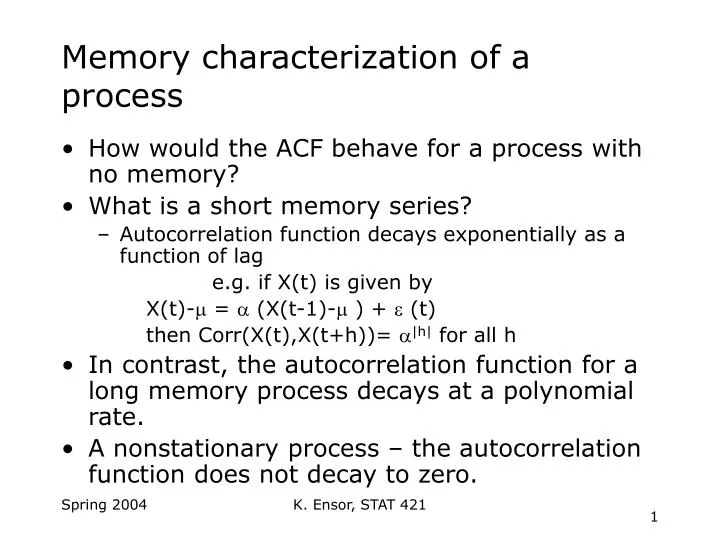
Memory characterization of a process • How would the ACF behave for a process with no memory? • What is a short memory series? • Autocorrelation function decays exponentially as a function of lag e.g. if X(t) is given by X(t)-m = a (X(t-1)-m ) + e (t) then Corr(X(t),X(t+h))= a|h| for all h • In contrast, the autocorrelation function for a long memory process decays at a polynomial rate. • A nonstationary process – the autocorrelation function does not decay to zero. K. Ensor, STAT 421
White noise • Uncorrelated OR independent random variables. • Identically distributed • Usually with mean 0, but must be finite • And variance finite variance 2 • Notation rt~ WN(0, 2) • What if we computed the ACF or PACF? K. Ensor, STAT 421
Linear Time Series • A time series rt if it can be written as a linear function of present and past values of a white noise series. rt= + jiat-j where j=0 to infinity and at is a white noise series. • The coefficients define the behavior of the series. • Let’s take a look at the mean and covariance for a covariance stationary (or weakly stationary) linear time series. K. Ensor, STAT 421
Autoregressive models • Just as the name implies, an autoregressive model is derived by regressing our process of interest on its on past. • Consider an autoregressive model of order 1, or AR(1) model or r(t)=0 + 1 r(t-1) + a(t) with a(t) representing a white noise process • Or more generally the AR(p) model where r(t)=0 + 1 r(t-1) + pr(t-p) a(t) K. Ensor, STAT 421
Characterisitics of an AR process • The behavior of the difference equation associated with the process determines the behavior of the process. Solutions to this equation are referred to as the characteristic roots. • Same comment about the behavior of the equation characterizing the autocorrelations. • The ACF decays exponentially to zero. • Recall ACF for AR(1) • The PACF is zero after the lag of the AR process (see section 2.4.2.) K. Ensor, STAT 421
Moving Average Model • Weighted average of present and past shocks to the system. r(t)=0 + 1 a(t-1) + a(t) with a(t) representing a white noise process • Or more generally the MA(q) model where r(t)= 0 + 1 a(t-1) + qa(t-q) + a(t) • Can also be viewed as a representation of an infinite or AR model. • Basic properties • Autocorrelation is zero after the largest lag of the process. • Partial autocorrelation decays to zero. K. Ensor, STAT 421
ARMA models • The series r(t) is a function of past values of itself plus current and past values of the noise or shocks to the system. • See page 50. • More next class period. K. Ensor, STAT 421