Download
1 / 21
210 likes | 361 Views
Prediction of a nonlinear time series with feedforward neural networks. Mats Nikus Process Control Laboratory. The time series. A closer look. Another look. Studying the time series. Some features seem to reapeat themselves over and over, but not totally ”deterministically”

E N D
Prediction of a nonlinear time series with feedforward neural networks Mats Nikus Process Control Laboratory
Studying the time series • Some features seem to reapeat themselves over and over, but not totally ”deterministically” • Lets study the autocovariance function
Studying the time series • The autocovariance function tells the same: There are certainly some dynamics in the data • Lets now make a phaseplot of the data • In a phaseplot the signal is plotted against itself with some lag • With one lag we get
The phase plots tell • Use two lagged values • The first lagged value describes a parabola • Lets make a neural network for prediction of the timeseries based on the findings.
The neural network ^ y(k+1) Lets try with 3 hidden nodes 2 for the ”parabola” and one for the ”rest” y(k) y(k-1)
A more difficult case • If the time series is time variant (i.e. the dynamic behaviour changes over time) and the measurement data is noisy, the prediction task becomes more challenging.
Use a Kalman-filter to update the weights • We can improve the predictions by using a Kalman-filter • Assume that the process we want to predict is described by
Kalman-filter • Use the following recursive equations The gradient needed in Ck is fairly simple to calculate for a sigmoidal network
Henon series • The timeseries is actually described by