Download
1 / 27
270 likes | 435 Views
Connectivity of aMRI and fMRI data. Keith Worsley Arnaud Charil Jason Lerch Francesco Tomaiuolo Department of Mathematics and Statistics, McConnell Brain Imaging Centre, Montreal Neurological Institute, McGill University. Effective connectivity.

E N D
Connectivity of aMRI and fMRI data Keith Worsley Arnaud Charil Jason Lerch Francesco Tomaiuolo Department of Mathematics and Statistics, McConnell Brain Imaging Centre, Montreal Neurological Institute, McGill University
Effective connectivity • Measured by the correlation between residuals at pairs of voxels: Activation only Correlation only Voxel 2 + + Voxel 2 + + + + + + + Voxel 1 + Voxel 1 + +
Types of connectivity • Focal • Extensive
3 2 1 0 -1 -2 -3 -2 0 2 Focal correlation 3 0 1 2 3 cor=0.58 2 1 4 5 6 7 0 -1 8 9 10 11 n = 120 frames -2 -3
Extensive correlation 3 0 1 2 3 cor=0.13 2 1 4 5 6 7 0 -1 8 9 10 11 -2 -3
Methods • Seed • Iterated seed • Thresholding correlations • PCA
Method 1: ‘Seed’ • Friston et al. (19??): Pick one voxel, then find all others that are correlated with it: • Problem: how to pick the ‘seed’ voxel?
Method 2: Iterated ‘seed’ • Problem: how to find the rest of the connectivity network? • Hampson et al., (2002): Find significant correlations, use them as new seeds, iterate.
Method 3: All correlations • Problem: how to find isolated parts of the connectivity network? • Cao & Worsley (1998): find all correlations (!) • 6D data, need higher threshold to compensate
Thresholds are not as high as you might think: E.g. 1000cc search region, 10mm smoothing, 100 df, P=0.05: dimensions D1 D2 Cor T Voxel1 - Voxel2 0 0 0.165 1.66 One seed voxel - volume 0 3 0.448 4.99 Volume – volume (auto-correlation) 3 3 0.609 7.64 Volume1 – volume2 (cross-correlation) 3 3 0.617 7.81
Practical details • Find threshold first, then keep only correlations > threshold • Then keep only local maxima i.e. cor(voxel1, voxel2) > cor(voxel1, 6 neighbours of voxel2), > cor(6 neighbours of voxel1, voxel2),
Method 4: Principal Components Analysis (PCA) • Friston et al: (1991): find spatial and temporal components that capture as much as possible of the variability of the data. • Singular Value Decomposition of time x space matrix: • Y = U D V’ (U’U = I, V’V = I, D = diag) • Regions with high score on a spatial component (column of V) are correlated or ‘connected’
Which is better: thresholding correlations, or PCA?
Summary Focal correlation Extensive correlation 6 6 0 1 2 3 0 1 2 3 4 4 Thresholding T statistic (=correlations) 2 2 4 5 6 7 4 5 6 7 0 0 -2 -2 8 9 10 11 8 9 10 11 -4 -4 -6 -6 1 1 0 1 2 3 0 1 2 3 0.8 0.8 0.6 0.6 0.4 0.4 PCA 4 5 6 7 4 5 6 7 0.2 0.2 0 0 -0.2 -0.2 -0.4 -0.4 8 9 10 11 8 9 10 11 -0.6 -0.6 -0.8 -0.8 -1 -1
First scan of fMRI data Highly significant effect, T=6.59 1000 hot 890 rest 880 870 warm 500 0 100 200 300 No significant effect, T=-0.74 820 hot 0 rest 800 T statistic for hot - warm effect warm 5 0 100 200 300 Drift 810 0 800 790 -5 0 100 200 300 Time, seconds fMRI data: 120 scans, 3 scans each of hot, rest, warm, rest, hot, rest, … T = (hot – warm effect) / S.d. ~ t110 if no effect
PCA of time space: Temporal components (sd, % variance explained) 1: exclude first frames 0 1 0.68, 46.9% 2 0.29, 8.6% 2: drift Component 3 0.17, 2.9% 4 0.15, 2.4% 5 0 20 40 60 80 100 120 Frame 3: long-range correlation or anatomical effect: remove by converting to % of brain Spatial components 1 1 0.5 2 0 Component 3 -0.5 4 -1 4: signal? 0 2 4 6 8 10 12 Slice (0 based)
MS lesions and cortical thickness(Arnaud et al., 2004) • n = 425 mild MS patients • Lesion density, smoothed 10mm • Cortical thickness, smoothed 20mm • Find connectivity i.e. find voxels in 3D, nodes in 2D with high cor(lesion density, cortical thickness)
n=425 subjects, correlation = -0.56826 5.5 5 4.5 4 Average cortical thickness 3.5 3 2.5 2 1.5 0 10 20 30 40 50 60 70 80 Average lesion volume
Normalization • Simple correlation: Cor( LD, CT ) • Subtracting global mean thickness: Cor( LD, CT – avsurf(CT) ) • And removing overall lesion effect: Cor( LD – avWM(LD), CT – avsurf(CT) )
threshold threshold threshold threshold
Deformation Based Morphometry (DBM) (Tomaiuolo et al., 2004) • n1 = 19 non-missile brain trauma patients, 3-14 days in coma, • n2 = 17 age and gender matched controls • Data: non-linear vector deformations needed to warp each MRI to an atlas standard • Locate damage: find regions where deformations are different, hence shape change • Is damage connected? Find pairs of regions with high canonical correlation.
T = sqrt(df) cor / sqrt (1 - cor2) 6 Seed 0 1 2 3 T max = 7.81 P=0.00000004 4 2 4 5 6 7 0 -2 8 9 10 11 -4 -6
PCA, component 1 1 0 1 2 3 0.8 0.6 0.4 4 5 6 7 0.2 0 -0.2 -0.4 8 9 10 11 -0.6 -0.8 -1
T, extensive correlation 6 Seed 0 1 2 3 T max = 4.17 P = 0.59 4 2 4 5 6 7 0 -2 8 9 10 11 -4 -6
PCA, focal correlation 1 0 1 2 3 0.8 0.6 0.4 4 5 6 7 0.2 0 -0.2 -0.4 8 9 10 11 -0.6 -0.8 -1
Modulated connectivity • Looking for correlations not very interesting – ‘resting state networks’ • More intersting: how does connectivity change with • task or condition (external) • response at another voxel (internal) • Friston et al., (1995): add interaction to the linear model: • Data ~ task + seed + task*seed • Data ~ seed1 + seed2 + seed1*seed2
Fit a linear model for fMRI time series with AR(p) errors • Linear model: • ? ? • Yt = (stimulust * HRF) b + driftt c + errort • AR(p) errors: • ? ? ? • errort = a1 errort-1 + … + ap errort-p + s WNt • Subtract linear model to get residuals. • Look for connectivity. unknown parameters