Mastering Digital Image Essentials
340 likes | 369 Views
Understand digital image representation, reading, writing, and storage fundamentals in MATLAB. Learn about image types, classes, and data manipulation techniques. Dive into pixel intensity, binary images, and array indexing. Enhance your M-function programming skills.

Mastering Digital Image Essentials
E N D
Presentation Transcript
Chapter 2 Fundamentals The images used here are provided by the authors. Objectives: Digital Image Representation Image as a Matrix Reading and Displaying Images Writing Images Storage Classes and Data Types Image Coordinate System Summary of on MATLAB
Chapter 2 Fundamentals 2.1 Digital Image Representation 2.1.1 Coordinate Conventions 2.1.2 Images as Matrices 2.2 Reading Images 2.3 Displaying Images 2.4 Writing Images 2.5 Data Classes 2.6 Image Types 2.6.1 Intensity Images 2.6.2 Binary Images 2.6.3 A Note on Terminology 2.7 Converting between Data Classes and Image Types 2.7.1 Converting between Data Classes 2.7.2 Converting between Image Classes and Types 2.8 Array Indexing 2.8.1 Vector Indexing 2.8.2 Matrix Indexing 2.8.3 Selecting Array Dimensions 2.9 Some Important Standard Arrays 2.10 Introduction to M-Function Programming 2.10.1 M-Files 2.10.2 Operators 2.10.3 Flow Control 2.10.4 Code Optimization 2.10.5 Interactive I/O 2.10.6 A Brief Introduction to Cell Arrays and Structures 62 Summary
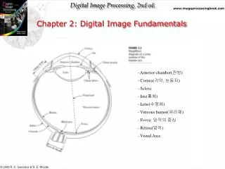
Chapter 2 Fundamentals Digital Image Fundamentals Lens is made of concentric layers of fibrous cells and is suspended by fibers that attach to the ciliary body. It contains 60% -70% water, 6% fat, and more protein than any other tissue in the eye. There are 6 to 7 million cones in each eye. Cones are located at the central portion of the retina. They are highly color sensitive. We use them to resolve fine details. Cone vision is called photopic or bright-light vision. There are 75-150 million rods distributed over the retinal surface. Larger area of distribution and the fact that several of rods are connected to a single nerve, make them less effective for resolving details. Rod vision is called scotopic or dim-light vision. Focal length 17 mm to about 14 mm
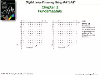
Chapter 2 Fundamentals Digital Image Representation An image can be seen as a two-dimensional function, f(x,y), where x and y are spatial (plane) coordinates, and the amplitude of f at any pair of coordinates (x,y) is called the intensity of the image at that point. This is an M-by-N image with indices starting from 0 This is an M-by-N image with indices starting from 1 (MATLAB Notation) The images used here are provided by the authors.
Chapter 2 Fundamentals Image as Matrices The image data can be represented as a matrix in the following form: Each element (building block) of an image is called a pixel. In MATLAB, the above matrix is represented as: This is how you store a 4-by-4 matrix as A in MATLAB: >> A = [1 5 9 13; 2 6 10 14; 3 7 11 15; 4 8 12 16] The images used here are provided by the authors.
Chapter 2 Fundamentals Reading and Displaying Images In MATLAB images are read using: imread(‘filename’). This reads the image that is stored in the current directory. We can include the path to a directory if that is different from the current directory: f = imread(‘D:\myimages\chestxray.jpg’) This reads the image chestxray.jpg from the D: drive and stores its data in matrix f. It is possible to read images of different formats as indicated in Table 2.1. The images used here are provided by the authors.
Chapter 2 Fundamentals Reading and Displaying Images Reading: >> f = imread(‘kids.tif’); Displaying: >> imshow(f) The whos function displays additional information: >> whos f Name Size Bytes Class f 400x318 127200 uint8 array Grand total is 127200 elements using 127200 bytes To keep the first image and output a second image, we will use: >> g = imread(‘trees.tif’); >> figure, imshow(g) Now, sine you had previously displayed the kids.tif, both the kids.tif and the trees.tif images will appear on the screen.
Chapter 2 Fundamentals Writing Images Assuming we have read an image already using: f = imread(‘greens.jpg). This is an image in jpg format. Images are written to disk using function imwrite, which is used as: imwrite(f, ‘filename’) Using this format, the string for filename MUST include a recognizable file format extension. We can also specify the desired format using: >> imwrite(f, ‘greens’, ‘tif’) Or >> imwrite(f, ‘greens.tif’) We can also write the image with a different quality defind as q%: imwrite(f, ‘greens_25.jpg’, ‘quality’, 25), where 25 is 25% quality Note: Quality only applies to images written in JPEG format because there is a compression associated with this format. We will discuss this later.
Chapter 2 Fundamentals Writing Images I used the iminfo command on the greens images of 100% and 25% qualities. Here are the result. Everything seems to be the same, so where does the size difference come from? K = imfinfo('greens_25.jpg') K = Filename: 'greens_25.jpg' FileModDate: '01-Mar-2001 09:52:40' FileSize: 22497 Format: 'jpg' FormatVersion: '' Width: 500 Height: 300 BitDepth: 24 ColorType: 'truecolor' FormatSignature: '' NumberOfSamples: 3 CodingMethod: 'Huffman' CodingProcess: 'Sequential' Comment: {} K = imfinfo('greens.jpg') K = Filename: 'greens.jpg' FileModDate: '01-Mar-2001 09:52:40' FileSize: 74948 Format: 'jpg' FormatVersion: '' Width: 500 Height: 300 BitDepth: 24 ColorType: 'truecolor' FormatSignature: '' NumberOfSamples: 3 CodingMethod: 'Huffman' CodingProcess: 'Sequential' Comment: {}
Chapter 2 Fundamentals Writing Images – how much we gained how much we lost? >> K=imfinfo('greens.jpg'); >> img_bytes = K.Width*K.Height*K.BitDepth/8; >> compressed_bytes = K.FileSize; >> compression_ratio = img_bytes/compressed_bytes compression_ratio = 6.0042 >> K=imfinfo('greens_25.jpg'); >> img_bytes = K.Width*K.Height*K.BitDepth/8; >> compressed_bytes = K.FileSize; >> compression_ratio = img_bytes/compressed_bytes compression_ratio = 20.0027
Chapter 2 Fundamentals Writing Images The images used here are provided by the authors.
Chapter 2 Fundamentals Writing Images The images used here are provided by the authors.
Chapter 2 Fundamentals Storage Classes By default, MATLAB stores most data in arrays of class double. The data in these arrays is stored as double-precision (64-bit) floating-point numbers. All MATLAB functions work with these arrays. For image processing, however, this data representation is not always ideal. The number of pixels in an image can be very large; for example, a 1000-by-1000 image has a million pixels. Since each pixel is represented by at least one array element, this image would require about 8 megabytes of memory. To reduce memory requirements, MATLAB supports storing image data in arrays as 8-bit or 16-bit unsigned integers, class uint8 and uint16. These arrays require one eighth or one fourth as much memory as double arrays.
Chapter 2 Fundamentals Data Classes The images used here are provided by the authors.
Chapter 2 Fundamentals Converting between Image Classes and types >> f = [-0.5 0.5; 0.75 1.5] f = -0.5 0.5 0.75 1.5 >> g = uint8(f) g = 0 1 1 2
Chapter 2 Fundamentals Image Types • The Image Processing Toolbox supports four basic types of images: • Indexed images • Intensity images • Binary images • RGB images • Reading a Graphics Image Writing a Graphics Image Querying a Graphics File Converting Image Storage Classes Converting Graphics File Formats Reading and Writing DICOM Files
Chapter 2 Fundamentals Coordinate Systems Pixel Coordinates Spatial Coordinates
Chapter 2 Fundamentals • Accessing Matrix Elements • Subscripts • Uses parentheses to indicate subscripts • A(1,4) + A(2,4) + A(3,4) + A(4,4) returns 34 • Out of range indices • Trying to read an element out of range produces an error message • Trying to assign a value to an element out of range expands the matrix !!A(5,4) = 17 produces 16 3 2 13 0 5 10 11 8 0 9 6 7 12 0 4 15 14 1 17
Chapter 2 Fundamentals The Colon Operator • Examples • 1:5 produces 1 2 3 4 5 • 20:-3:0 produces 20 17 14 11 8 5 2 • 0:pi/4:pi produces 0 0.7854 1.5708 2.3562 3.1416 • Accessing portions of a matrix • A(1:k,j) references the first k elements in the j column • A(:,end) references all elements in the last column • How could you reference all elements in the last row?
Chapter 2 Fundamentals Example: >> f = imread('kids.tif'); >> imshow(f) >> fp = f(end:-1:1, :); This command, flips the image vertically >> imshow(fp)
Chapter 2 Fundamentals Example: >> fc = f(100:300, 100:300); This cuts the pixels from 100 to 300 out from the original image, f. >> imshow(fc) >> fs = f(1:2:end, 1:2:end); This command create a subsampled image shown below. >> imshow(fs) >> plot(f(200,:) ) This plots a horizontal scan line through row 200, almost the middle.
Chapter 2 Fundamentals Expressions and Functions • Expressions and functions obey algebraic rulesz = sqrt(besselk(4/3,rho-i))z = 0.3730+ 0.3214i • Some important constant functions
Generating Matrices Chapter 2 Fundamentals randn produces normally distributed random numbers
Chapter 2 Fundamentals Various Matrix Operations - 1 • Concatenation, using our magic square A • This isn’t a magic square but the columns add up to the same value
Chapter 2 Fundamentals Various Matrix Operations - 2 • Deleting rows and columns • A(: , 2) = [ ] removes the second column • How would you remove the last row? • Single elements can only be removed from vectors • Some operations with transpose • If you tried to apply the determinant operation, you would find det(A) = 0, so this matrix is not invertible; if you tried inv(A) you would get an error
Chapter 2 Fundamentals Various Matrix Operations - 3 • The eigenvalue contains a 0, indicating singularity • P = A/34 is doubly stochastic, as shown above • P^5 (raised to the fifth power) converges towards ¼, as k in p^k gets larger the values approach ¼
Chapter 2 Fundamentals Array Operations • For example, to square the elements of A, enter the expression A.*A
Chapter 2 Fundamentals Building Tables • An example • Let n = (0:9)’ • Let pows = [n n.^2 2.^n] • Another example
Chapter 2 Fundamentals Programming in MATLAB • Control structures • Selection (if and switch) • Repetition (for, while, break, continue) • Other (try … catch, return) • Dynamic Structures • Scripts and M files • User defined functions • Two examples • Finding the periodicity of sunspots • Multiplying polynomials using FFT
Chapter 2 Fundamentals The if command • An example Useful Boolean tests for matrices
Chapter 2 Fundamentals The switch command • Note: the break command in C++ is not required in MATLAB
Chapter 2 Fundamentals Commands for repetition • The for command (notice the required ‘end’) • The while command (also requires ‘end’) Does anyone recognize what this code fragment does?
Chapter 2 Fundamentals Continue and Break What does this code fragment do? • The continue command • The break command Here is the finding the solution of a polynomial using bisection; why is the ‘break’ command an improvement?
Chapter 2 Fundamentals try … catch and return You can examine the error using lasterr An error in the exception handler causes the program to terminate • The return command • Terminates execution • If inside a user defined function, returns to the calling environment • Otherwise returns to keyboard input