Download
1 / 112
1.12k likes | 1.15k Views
CompuCell3D is a versatile modeling environment great for developing GGH-based simulations. Learn about its advantages, architecture, programming languages, and visualization tools. Discover how CompuCell3D simplifies simulations and promotes collaboration worldwide.

E N D
Introduction to CompuCell3D • Outline: • What is CompuCell3D? • Why use CompuCell3D? • Demo simulations • Glazier-Graner-Hogeweg (GGH) model – an overview • CompuCell3D architecture and terminology • XML 101 • Building first CompuCell3D simulation • Visualization package – CompuCell Player • Python scripting inside CompuCell3D
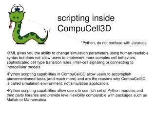
What Is CompuCell3D? • CompuCell3D is a modeling environment used to build, test, run and visualize GGH-based simulations • CompuCell3D has built-in scripting language (Python) that allows users to quite easily write extension modules that are essential for building sophisticated biological models. • CompuCell3D thus is NOT a specialized software • Running CompuCell3D simulations DOES NOT recompilation • CompuCell3D model is described using CompuCell3D XML syntax and in the case of using Python language , a Python script(s) • CompuCell3D platform is distributed with a GUI front end – CompuCell Player or simply Player. The Player provides 2- and 3-D visualization capabilities. • Models developed by one CompuCell3D user can be “replayed” by another user regardless the operating system/hardware on which CompuCell is installed. • CompuCell3D is a cross platform application with Windows port being currently developed (due end of July 2007).
Why Use CompuCell3D? What Are the Alternatives? • CompuCell3D allows users to set up and run their simmulations within minutes, maybe hours. A typical development of a specialized GGH code takes orders of magnitudes longer time. • CompuCell3D simulations DO NOT need to be recompiled. If you want to change parameters (in XML or Python scripts) or logic (in Python scripts) you just make the changes and re-run the simulation. With hand-compiled simulations there is much more to do. Recompilation of every simulation is also error prone and often limits users to those who have significant programming background. • CompuCell3D is actively developed , maintained and supported. On www.compucell3d.org website users can download manuals, tutorials and developer documentation. CompuCell3D has approx. 10 releases each year. • CompuCell3D has many users around the world. This makes it easier to collaborate or exchange modules and results saving time spent on developing new model. • The Biocomplexity Institute organizes training workshops and mentorship programs. Those are great opportunities to visit Bloomington and learn biological modeling using CompuCell3D. For more info see www.compucell3d.org
The GGH Model – an Overview x 20 • Energy minimization formalism • - extended by Graner and Glazier, 1992 • DAH: Contact energy depending on cell types (differentiated cells) • Metropolis algorithm: probability of configuration change
Brief Explanation of Equation Symbols s(x) –denotes id of the cell occupying position x. All pixels pointed by arrow have same cell id , thus they belong to the same cell t(s(x)) denotes cell type of cell with id s(x). In the picture above blue and yellow cells have different cell types and different cell id. Arrows mark different cell types Notice that in your model you may (will) have many cells of the same type but with different id. For example in a simple cellsorting simulation there will be many cells of type “Condensing” and many cells with type “NonCondensinig”
CompuCell3D Architecture Object oriented implementation in C++ and Python Visualization, Steering, User Interface Plugins Calculate change in energy Python Interpreter Biologo Code Generator Kernel Runs Metropolis Algorithm PDE Solvers Lattice monitoring
Typical “Run-Time” Architecture of CompuCell • CompuCell can be run in a variety of ways: • Through the Player with or without Python interpreter • As a Python script • As a stand alone computational kernel+plugins CompuCellPlayer Python CompuCell3D Kernel Plugins
CompuCell3D terminology • Spin-copy attempt is an event where program randomly picks a lattice site in an attempt to copy its spin to a neighboring lattice site. • Monte Carlo Step (MCS) consists of series spin-copy attempts. Usually the number of spin copy-attempts in single MCS is equal to the number of lattice sites, but this is can be customized • CompuCell3D Plugin is a software module that either calculates an energy term in a Hamiltonian or implements action in response to spin copy (lattice monitors). Note that not all spin-copy attempts will trigger lattice monitors to run. • Steppables are CompuCell3D modules that are run every MCS after all spin-copy attempts for a given MCS have been exhausted. Most of Steppables are implemented in Python. Most customizations of CompuCell3D simulations is done through Steppables • Steppers are modules that are run for those spin-copy attempts that actually resulted in energy calculation. They are run regardless whether actual spin-copy occurred or not. For example cell mitosis is implemented in the form of stepper. • Fixed Steppers are modules that are run every spin-copy attempt.
CompuCell3D Terminology – Visual Guide Change pixel Spin copy “blue” pixel (newCell) replaces “yellow” pixel (oldCell) 100x100x1 square lattice = 10000 lattice sites (pixels) MCS 21 MCS 22 MCS 23 MCS 24 10000 spin-copy attempts 10000 spin-copy attempts 10000 spin-copy attempts 10000 spin-copy attempts Run Steppables Run Steppables Run Steppables
Nearest neighbors in 2D and their Euclidian distances from the central pixel 3 5 4 4 5 4 1 2 2 4 1 3 1 3 1 2 4 4 2 3 4 4 5 5 Spin copy can take place between any order nearest neighbor (although in practice we limit ourselves to only few first oders). <FlipNeighborMaxDistance>1.45</FlipNeighborMaxDistance> 2nd nearest neighbor Contact energy calculation (see further slides) are also done up to certain order of nearest neighbors (default is 1) <Depth>2.1</Depth>
XML 101 XML stands for eXtensible Markup Manguage. It is NOT a programming language. Its main purpose is to standarize information exchange between different applications. XML Example: <Sentence> <Text>It is too early to be in class</Text> <FontType>TimesNewRoman</FontType> <FontSize>12</FontSize> <DisplayHint Hint=“AddFrameAround”/> </Sentence>
CompuCell Related Example Defining basic properties of the simulation like lattice dimension, number of Monte Carlo Steps, Temperature and ratio of spin-copy attempts to number of lattice sites (Flip2DimRatio). <Potts> section has to be included in every CompuCell3D simulation <Potts> <Dimensionsx="71" y="36" z="211"/> <Steps>10</Steps> <Temperature>2</Temperature> <Flip2DimRatio>2</Flip2DimRatio> </Potts> Defining properties of Volume Energy term – cell target volume and lambda parameter: <PluginName=“Volume"> <TargetVolume>25</TargetVolume> <LambdaVolume>2.0</LambdaVolume> </Plugin> ...
Building Your First CompuCell3D Simulation Cell All simulation parameters are controlled by the config file. The config file allows you to only add those features needed for your current simulation, enabling better use of system resources. Define Lattice and Simulation Parameters < CompuCell3D> <Potts> <Dimensionsx=“100" y=“100" z=“1"/> <Steps>10</Steps> <Temperature>2</Temperature> <Flip2DimRatio>1</Flip2DimRatio> </Potts> … </CompuCell3D>
Cell Define Cell Types Used in the Simulation Each CompuCell3D xml file must list all cell types that will used in the simulation <Plugin Name="CellType"> <CellType TypeName="Medium" TypeId="0"/> <CellType TypeName=“Light" TypeId="1"/> <CellType TypeName=“Dark" ="2"/> </Plugin> Notice that Medium is listed with TypeId =0. This is both convention and a REQUIREMENT in CompuCell3D. Reassigning Medium to a different TypeId may give undefined results. This limitation will be fixed in one of the next CompuCell3D releases
Cell Define Energy Terms of the Hamiltonian and Their Parameters Volume volume volumeEnergy(cell) <Plugin Name="Volume"> <TargetVolume>25</TargetVolume> <LambdaVolume>1.0</LambdaVolume> </Plugin> <Plugin Name="Surface"> <TargetSurface>21</TargetSurface> <LambdaSurface>0.5</LambdaSurface> </Plugin> Surface area surfaceEnergy(cell) <Plugin Name="Contact"> <Energy Type1="Medium" Type2="Medium">0 </Energy> <Energy Type1="Light" Type2="Medium">0 </Energy> <Energy Type1="Dark" Type2="Medium">0.1 </Energy> <Energy Type1="Light" Type2="Light">0.5 </Energy> <Energy Type1="Dark" Type2="Dark">3.0 </Energy> <Energy Type1="Light" Type2="Dark">0.5 </Energy> </Plugin> Contact contactEnergy( cell1, cell2)
Plugin XML Syntax <Plugin Name="Volume"> <TargetVolume>25</TargetVolume> <LambdaVolume>1.0</LambdaVolume> </Plugin> <Plugin Name="Surface"> <TargetSurface>21</TargetSurface> <LambdaSurface>0.5</LambdaSurface> </Plugin>
Plugin XML Syntax – Contact Energy <Plugin Name="Contact"> <Energy Type1="Medium" Type2="Medium">0 </Energy> <Energy Type1="Light" Type2="Medium">0 </Energy> <Energy Type1="Dark" Type2="Medium">0.1 </Energy> <Energy Type1="Light" Type2="Light">0.5 </Energy> <Energy Type1="Dark" Type2="Dark">3.0 </Energy> <Energy Type1="Light" Type2="Dark">0.5 </Energy> </Plugin> 1-d term ensures that pixels belonging to the same cell do not contribute to contact energy
Laying Out Cells on the Lattice Using built-in cell field initializer: <Steppable Type="BlobInitializer"> <Gap>0</Gap> <Width>5</Width> <CellSortInit>yes</CellSortInit> <Radius>40</Radius> </Steppable> This is just an example of cell field initializer. More general ways of cell field initialization will be discussed later.
Putting It All Together - cellsort_2D.xml <CompuCell3D> <Potts> <Dimensions x="100" y="100" z="1"/> <Steps>10</Steps> <Temperature>2</Temperature> <Flip2DimRatio>1</Flip2DimRatio> </Potts> <Plugin Name="CellType"> <CellType TypeName="Medium" TypeId="0"/> <CellType TypeName=“Light" TypeId="1"/> <CellType TypeName=“Dark" ="2"/> </Plugin> <Plugin Name="Volume"> <TargetVolume>25</TargetVolume> <LambdaVolume>1.0</LambdaVolume> </Plugin> <Plugin Name="Surface"> <TargetSurface>21</TargetSurface> <LambdaSurface>0.5</LambdaSurface> </Plugin> <Plugin Name="Contact"> <Energy Type1="Medium" Type2="Medium">0 </Energy> <Energy Type1="Light" Type2="Medium">0 </Energy> <Energy Type1="Dark" Type2="Medium">0.1 </Energy> <Energy Type1="Light" Type2="Light">0.5 </Energy> <Energy Type1="Dark" Type2="Dark">3.0 </Energy> <Energy Type1="Light" Type2="Dark">0.5 </Energy> </Plugin> <Steppable Type="BlobInitializer"> <Gap>0</Gap> <Width>5</Width> <CellSortInit>yes</CellSortInit> <Radius>40</Radius> </Steppable> </CompuCell3D> Coding the same simulation in C/C++/Java/Fortran would take you at least 1000 lines of code…
Putting It All Together - Avoiding Common Errors in XML code • First specify Potts section, then list all the plugins and finally list all the steppables. This is the correct order and if you mix e.g. plugins with steppables you will get an error. Remember the correct order is • Potts • Plugins • Steppables • 2. Remember to match every xml tag with a closing tag • <Plugin> • … • </Plugin> • 3. Watch for typos • 4. Modify available examples rather than starting from scratch
CompuCellPlayer – the Best Way To Run Simulations Steering bar allows users to start or pause the simulation, zoom in , zoom out, to switch between 2D and 3D visualization, change view modes (cell field, pressure field , chemical concentration field, velocity field etc..) Player can output multiple views during single simulation run – Add Screenshot function Information bar
Opening a Simulation in the Player Go to File->Open Simulation ; Click Simulation xml file -> Browse… button
Running Simulation From Command Line You can simply start the simulation with or without Player straight from command line Open up console (terminal) and type: ./compucell3d.command –i cellsort_2D.xml (on OSX) ./compucell3d.command –i cellsort_2D.xml (on Linux) Running CompuCell3D from command line not only convenient, but sometimes (on clusters) the only option to run the simulation. For more information about command line options please see “Running CompuCell3D” manual available at www.compucell3d.org.
Running the Simulation • After typing the XML file in your favorite editor all you need to do to run the simulation is to open the XML file in the Player and hit “Play” button. • Screenshots from the simulations are automatically stored in the directory with name composed of simulation file name and a time at which simulation was started • As you can see this setting CompuCell3D simulation was reasonably simple. • It is quite likely that if you were to code entire simulation in C/C++/Java etc. you would need much more time. • We hope that now you understand why using CompuCell3D saves you a lot of time and allows you to concentrate on biological modeling and not on writing low level computer code. • During last year we have improved CompuCell3D performance so that it is on par with hand-written code. Yet, if you really to have the fastest GGH code in the world you should write code your own simulation directly in C or even better in assembly language. Before you do it, make sure you want to spend time rewriting the code that already exist. We hope you will enjoy CompuCell3D and for more information please visit www.compucell3d.org.
Capabilities of CompuCellPlayer • Provides wide range of visualization - cell field plots, concentration plots, vector field plots in both 2- and 3-D • Allows to store multiple lattice views in a single run. For example users can store multiple projections of the cell lattice, concentration fields, various 3D views etc… in a single run. • Can be run in GUI and silent mode (i.e. without displaying GUI but still saving screenshots) • Is ready to be used on clusters that do not have X-server installed. This feature is essential for doing “production runs” of your simulations. • Concentration fields and vector fields initialized from Python level can easily be displayed in the Player • Configurable from XML level for those users who prefer typing to clicking
XML initializers - UniformInitializer You may initialize simple geometries of cell clusters directly from XML <Steppable Type=“UniformInitializer"> <Region> <BoxMin x=“10” y=“10” z=“0”/> <BoxMax x=“90” y=“90” z=“1”/> <Types>Condensing,NonCondensing</Types> <Gap>0</Gap> <Width>5</Width> </Region> </Steppable> Specify box size and position Specify cell types – here the box will be filled with cells whose types are randomly chosen (either 1 or 2) Choose cell size and space between cells
<Steppable Type=“UniformInitializer"> <Region> <BoxMin x=“10” y=“10” z=“0”/> <BoxMax x=“90” y=“90” z=“1”/> <Types>Condensing</Types> <Gap>0</Gap> <Width>5</Width> </Region> </Steppable> Notice, we have only specified one type (Condensing) thus all the cells are of the same type
<Steppable Type=“UniformInitializer"> <Region> <BoxMin x=“10” y=“10” z=“0”/> <BoxMax x=“90” y=“90” z=“1”/> <Types>Condensing,NonCondensing</Types> <Gap>2</Gap> <Width>5</Width> </Region> </Steppable> Introducing a gap between cells
<Steppable Type="UniformInitializer"> <Region> <BoxMin x="10" y="10" z="0"/> <BoxMax x="40" y="40" z="1"/> <Gap>0</Gap> <Width>5</Width> <Types>Condensing,NonCondensing</Types> </Region> <Region> <BoxMin x="50" y="50" z="0"/> <BoxMax x="80" y="80" z="1"/> <Gap>0</Gap> <Width>3</Width> <Types>Condensing</Types> </Region> </Steppable> Notice, we have defined two regions with different cell sizes and different types
XML initializers - BlobInitializer <Steppable Type="BlobInitializer"> <Region> <Radius>30</Radius> <Center x="40" y="40" z="0"/> <Gap>0</Gap> <Width>5</Width> <Types>Condensing,NonCondensing</Types> </Region> <Region> <Radius>20</Radius> <Center x="80" y="80" z="0"/> <Gap>0</Gap> <Width>3</Width> <Types>Condensing</Types> </Region> </Steppable> Defining two regions with different cell sizes and different types for BlobInitializer is very similar to the same task with UniformInitilizer. There are some new XML tags which differ the two initializers.
Using PIFInitilizer Use PIFInitializer to create sophisticated initial conditions. PIF file allows you to compose cells from single pixels or from larger rectangular blocks The syntax of the PIF file is given below: Cell_id Cell_type x_low x_high y_low y_high z_low z_high Example (file: amoebae_2D_workshop.pif): 0 amoeba 10 15 10 15 0 0 This will create rectangular cell with x-coordinates ranging from 10 to 15 (inclusive), y coordinates ranging from 10 to 15 (inclusive) and z coordinates ranging from 0 to 0 inclusive. 0,0 <Steppable Type="PIFInitializer"> <PIFName>amoebae_2D_workshop.pif</PIFName> </Steppable>
Let’s add another cell: Example (file: amoebae_2D_workshop.pif): 0 Amoeba 10 15 10 15 0 0 1 Bacteria 35 40 35 40 0 0 Notice that new cell has different cell_id (1) and different type (Bacterium) Let’s add pixels and blocks to the two cells from previous example: Example (file: amoebae_2D_workshop.pif): 0 Amoeba 10 15 10 15 0 0 1 Bacteria 35 40 35 40 0 00 Amoeba 16 16 15 15 0 0 1 Bacteria 35 37 41 45 0 0 To add pixels, start new pif line with existing cell_id (0 or 1 here ) and specify pixels.
This is what happens when you do not reuse cell_id Example (file: amoebae_2D_workshop.pif): 0 Amoeba 10 15 10 15 0 0 1 Bacteria 35 40 35 40 0 00 Amoeba 16 16 15 15 0 0 2 Bacteria 35 37 41 45 0 0 Introducing new cell_id (2) creates new cell. PIF files allow users to specify arbitrarily complex cell shapes and cell arrangements. The drawback is, that typing PIF file is quite tedious task and , not recommended. Typically PIF files are created using scripts. In the future release of CompuCell3D users will be able to draw on the screen cells or regions filled with cells using GUI tools. Such graphical initialization tools will greatly simplify the process of setting up new simulations. This project has high priority on our TO DO list.
PIFDumper - yet another way to create initial condition PIFDumper is typically used to output cell lattice every predefined number of MCS. It is useful because, you may start with rectangular cells, “round them up” by running CompuCell3D , output cell lattice using PIF dumper and reload newly created PIF file using PIFInitializer. <Steppable Type="PIFDumper“ Frequency=“100”> <PIFName>amoebae</PIFName> </Steppable> Above syntax tells CompuCell3D to store cell lattice as a PIF file every 100 MCS. The files will be named amoebae.100.pif , amoebae.200.pif etc… To reload file , say amoebae.100.pif use already familiar syntax: <Steppable Type="PIFInitializer"> <PIFName>amoebae.100.pif</PIFName> </Steppable>
Practical way of guessing contact energy hierarchy • Basic facts: • Cells that have high contact energies between themselves, when they come together they increase overall energy of the system. • Cells that have low contact energies between themselves, when they come together they decrease overall energy of the system. • Those two rules are helpful when determining contact energy hierarchy. Simply cells of one type like to be surrounded by those cells with which the contact energy is the lowest. • And vice versa, if you want to make two cells not to touch each other, make sure that contact energy between them is high.
Examples of different contact energy hierarchies Cell sorting simulation where cells of both type like to be surrounded by medium. That is contact energy between Condensing and Medium as well as between NonCondensing and Medium is very low JCM=JNM<JNN<JCC<JNC
Examples of different contact energy hierarchies Cell sorting simulation where cells of both type do not like to be surrounded by medium and cells of homotypic cells do not like each other JNM<<JNN=JCC<JCM=JNM
Chemotaxis • Basic facts • Chemotaxis is defined as cell motion induced by a presence (gradient) of a chemical. • In GGH formalism chemotaxis is implemented as a spin copy bias which depends on chemical gradient. • Chemotaxis was first introduced to GGH formalism by Paulien Hogeweg from University of Utrecht, Netherlands • In CompuCell3D Chemotaxis plugin provides wide range of options to support different modes of chemotaxis. • Chemotaxis plugin requires the presence of at least one concentration field. The fields can be inserted into CompuCell3D simulation by means PDE solvers or can be created, initialized and managed explicitly from the Python level
Chemotaxis Term – Most Basic Form If concentration at the spin-copy destination pixel (c(xdestination)) is higher than concentration at the spin-copy source (c(xsource)) AND l is positive then DE is negative and such spin copy will be accepted. The cell chemotacts up the concentration gradient C(x) Lower concentration Higher concentration x Chemorepulsion can be obtained by making l negative
Chemotaxis - XML Examples <Plugin Name="Chemotaxis"> <ChemicalField Source="FlexibleDiffusionSolverFE" Name="FGF"> <ChemotaxisByType Type="Amoeba" Lambda="300"/> <ChemotaxisByType Type="Bacteria" Lambda="200"/> </ChemicalField> <ChemicalField Source="FlexibleDiffusionSolverFE" Name="FGF4"> <ChemotaxisByType Type="Amoeba" Lambda=“-300"/> </ChemicalField> </Plugin> Notice , that different cell types may have different chemotactic properties. For more than 1 chemical fields the change of chemotaxis energy expression is given below:
Chemotaxis - XML Examples continued <Plugin Name="Chemotaxis"> <ChemicalField Source="FlexibleDiffusionSolverFE" Name="FGF"> <ChemotaxisByType Type="Amoeba" Lambda="300"/> <ChemotaxisByType Type="Bacteria" Lambda="200"/> </ChemicalField> <ChemicalField Source="FlexibleDiffusionSolverFE" Name="FGF4"> <ChemotaxisByType Type="Amoeba" Lambda=“-300“ SaturationCoef=“2.0”/> </ChemicalField> </Plugin>
Chemotaxis - XML Examples continued <Plugin Name="Chemotaxis"> <ChemicalField Source="FlexibleDiffusionSolverFE" Name="FGF"> <ChemotaxisByType Type="Amoeba" Lambda="300"/> <ChemotaxisByType Type="Bacteria" Lambda="200"/> </ChemicalField> <ChemicalField Source="FlexibleDiffusionSolverFE" Name="FGF4"> <ChemotaxisByType Type="Amoeba" Lambda=“-300“ SaturationLinearCoef=“2.0”/> </ChemicalField> </Plugin>
PDE Solvers • CompuCell3D has built-in diffusion , reaction diffusion and advection diffusion PDE solvers. Those are, probably most frequently used solver in GGH modeling. • CompuCell3D uses explicit (unstable but fast) method to solve the PDE. Constantly changing boundary conditions practically rule out more robust, but slow implicit solvers. • Because of instability users should make sure that their PDE parameters do not produce wrong results (which could manifest themselves as “rough” concentration profiles, “insane” concentration values, NaN’s - Not A Number etc…). Future release of CompuCell3D will provide tools to detect potential PDE instabilities. • Additional solvers can be implemented directly in C++ or using BioLogo. BioLogo is especially attractive because it takes as an input human readable PDE description and generates fast C++ code. • Typically a concentration from the PDE solver is read by other CompuCell3D modules to adjust cell properties. Currently the best way of dealing with this is through Python interface.
Flexible Diffusion Solver <Steppable Type="FlexibleDiffusionSolverFE"> <DiffusionField> <DiffusionData> <FieldName>FGF</FieldName> <DiffusionConstant>0.010</DiffusionConstant> <DecayConstant>0.000</DecayConstant> <ConcentrationFileName>diffusion_2D.pulse.txt</ConcentrationFileName> </DiffusionData> </DiffusionField> </Steppable> Define diffusion field Define diffusion parameters Read-in initial condition Initial Condition File Format: x y z concentration Example: 27 27 0 2000.0 45 45 0 0.0 …
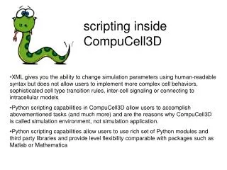
Two-pulse initial condition Initial condition (diffusion_2D.pulse.txt): 5 5 0 1000.0 27 27 0 2000.0
<Steppable Type="FlexibleDiffusionSolverFE"> <DiffusionField> <DiffusionData> <FieldName>FGF</FieldName> <DiffusionConstant>0.010</DiffusionConstant> <DecayConstant>0.000</DecayConstant> <DoNotDiffuseTo>Medium</DoNotDiffuseTo> <ConcentrationFileName>diffusion_2D.pulse.txt</ConcentrationFileName> </DiffusionData> </DiffusionField> </Steppable> You may specify diffusion regions FGF will diffuse inside big cell and will not go to Medium
<Steppable Type="FlexibleDiffusionSolverFE"> <DiffusionField> <DiffusionData> <FieldName>FGF</FieldName> <DiffusionConstant>0.010</DiffusionConstant> <DecayConstant>0.000</DecayConstant> <DoNotDiffuseTo>Wall</DoNotDiffuseTo> <ConcentrationFileName>diffusion_2D_wall.pulse.txt</ConcentrationFileName> </DiffusionData> </DiffusionField> </Steppable> FGF will not diffuse to the Wall