Download
1 / 41
410 likes | 722 Views
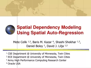
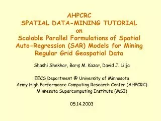
AHPCRC SPATIAL DATA-MINING TUTORIAL on Scalable Parallel Formulations of Spatial Auto-Regression (SAR) Models for Mining Regular Grid Geospatial Data . Shashi Shekhar, Barış M. Kazar, David J. Lilja EECS Department @ University of Minnesota

E N D
AHPCRCSPATIAL DATA-MINING TUTORIALonScalable Parallel Formulationsof Spatial Auto-Regression (SAR) Models for Mining Regular Grid Geospatial Data Shashi Shekhar, Barış M. Kazar, David J. Lilja EECS Department @ University of Minnesota Army High Performance Computing Research Center (AHPCRC) Minnesota Supercomputing Institute (MSI) 05.14.2003
Outline • Motivation for Parallel SAR Models • Background on Spatial Auto-regression Model • Our Contributions • Problem Definition & Hypothesis • Introduction to the SAR Software • Experimental Design • Related Work • Conclusions and Future Work AHPCRC Spatial Data-Mining Tutorial
Motivation for Parallel SAR Models • Linear regression models make the assumption of independent identical distribution (a.k.a. iid) about learning data samples. • Therefore, low prediction accuracy occurs • SAR model = generalization of linear regression model with an auto-correlation term • Incorporating the auto-correlation term: • Results in better prediction accuracy • However, computational complexity increases due to the logarithm-determinant (a.k.a. Jacobian) term of the maximum likelihood estimation procedure • Parallel processing can reduce execution time AHPCRC Spatial Data-Mining Tutorial
Our Contributions • This study is the first study that offers the only available parallel SAR formulation and evaluates its scalability • All of the eigenvalues of any type of dense neighborhood (square) matrix can be computed in parallel • Scalable parallel formulations of spatial auto-regression (SAR) models for 1-D and 2-D location prediction problems for planar surface partitionings using the eigenvalue computation • Hand-parallelized EISPACK, pre-parallelized LAPACK-based NAG linear algebra libraries and shared-memory parallel programming, i.e. OpenMP are used AHPCRC Spatial Data-Mining Tutorial
Background on Spatial Autoregression Model • Mixed Regressive Spatial Auto-regressive (SAR) Model where: y: n-by-1 vector of observations on dependent variable : spatial autoregression parameter (coefficient) W: n-by-n matrix of spatial weights (i.e. contiguity, neighborhood matrix) X: n-by-k matrix of observations on the explanatory variables : k-by-1 vector of regression coefficients I: n-by-n Identity matrix : n-by-1 vector of unobservable error term ~ N(0,2I) : common variance of error term • When = 0,the SAR model collapses to the classical regression model AHPCRC Spatial Data-Mining Tutorial
Background on SAR Model –Cont’d • If x= 0 and W2= 0, then first-order spatial autoregressive model is obtained as follows: y = W1y + ~ N(0, 2I) • If W2= 0, then mixed regressive spatial autoregressive model(a.k.a. spatial lag model) is obtained as follows: y = W1y + x + ~ N(0, 2I) • If W1= 0, then regression model with spatial autocorrelation inthe disturbances (a.k.a.spatial error model) is obtained as follows: y = x + u u = W2u + ~ N(0, 2I) AHPCRC Spatial Data-Mining Tutorial
Problem Definition • Given: • A Sequential solution procedure: “Serial Dense Matrix Approach” • Same as Prof. Bin Li’s method in Fortran 77 • Find: • Faster serial formulation called as “Serial Sparse Matrix Approach” • New Parallel Formulation of Serial Dense Matrix Approach different from Prof. Bin Li’s method in CM-fortran • Constraints: N(0,2I) IID • Rastor Data (resulting in binary neighborhood,contiguity matrix W) • Parallel Platform (HW: Origin 3800, IBM SP, IBM Regatta, Cray X1; SW: Fortran, OpenMP) • Size of W (big vs. small and dense vs. sparse) • Objective: • Maximize speedup (Tserial/Tparallel) • Scalability- Better than (Li,1996)’s formulation AHPCRC Spatial Data-Mining Tutorial
Hypotheses • There are a number of sequential algorithms computing SAR model, most of which are based on the estimation of maximum likelihood method that solves for the spatial autoregression parameter () andregression coefficients (). • As the problem size gets bigger, the sequential methods are incapable of solving this problem due to • extensive number of computations and • large memory requirement. • The new parallel formulation proposed in this study will outperform the previous parallel implementation in terms of: • Speedup (S), • Scalability, • Problem size (PS) and, • Memory requirement. AHPCRC Spatial Data-Mining Tutorial
Serial SAR Model Solution • Starting with normal density function: • The maximum likelihood (ML) function: • The explicit form of maximum likelihood (ML) function: AHPCRC Spatial Data-Mining Tutorial
Serial SAR Model Solution - (Cont’d) • The logarithm of the maximum likelihood function is called • log-likelihood function • The ML estimates of the SAR parameters: • The function to optimize: AHPCRC Spatial Data-Mining Tutorial
System Diagram Pre-processing Step B Golden Section Search to find that minimizes ML function C Compute and given the best estimate using least squares The Symmetric Eigenvalue-equivalent Neighborhood Matrix Eigenvalues ofW A Compute Eigenvalues Calculate the ML function AHPCRC Spatial Data-Mining Tutorial
Introduction to SAR Software • Following slides will describe: • how we implemented the SAR model solution • execution trace • Matlab is good for small size problems • Memory is not enough • Execution time is too long • Compiler language needed for larger problems such as Fortran • Up to 80GB can be used on supercomputers • Execution time decreased considerably due to parallel processing AHPCRC Spatial Data-Mining Tutorial
1. Pre-processing Step • It consists of four sub-steps • Forming Epsilon () Vector • Form W, the row-normalized Neighborhood Matrix • Symmetrize W • Form y & x Vectors Form Training Data Set y To box B Symmetrization of W FormW To box A AHPCRC Spatial Data-Mining Tutorial
1.0 Form Epsilon () Vector • Input: p=4; q=4; n=pq=16; • Output: a 16-by-1 column vector (epsilon) • The term i.e. the 16-by-1 vector of unobservable error term ~ N(0, 2I)in the SAR equation y = Wy + x + The elements are IID with zero mean and unit standard deviation normal random numbers • Prof. Isaku Wada’s normal random number generator written in C is used, which is much better than Matlab’s nrand function • T=[0.9914 -1.2780 -0.4976 1.2271 0.4740 -0.0700 0.0834 -0.8789 0.3378 -1.5901 0.0638 -0.2717 2.3235 -0.2973 -0.1964 0.1416] AHPCRC Spatial Data-Mining Tutorial
1.1 Form W, the Neighborhood Matrix • Input: p=4; q=4; n=pq=16; neighborhood type (4- Neighbors) • Output: The binary (non-row-normalized) 16-by-16 C matrix; the row-sum in a 16-by-1 column vector D_onehalf; the row-normalized 16-by-16 neighborhood matrix W • The neighborhood matrix, W is formed by using the following neighborhood relationship ((i.j) is the current pixel): • The solution can handle more cases such as: • 1-D 2-neighbors • 2-D 8,16,24 etc. neighbors AHPCRC Spatial Data-Mining Tutorial
6th row 6th row 1.1 Matrices for 4-by-4 Regular Grid Space (a) (b) (c) • (a) The spatial framework which is p-by-q (4-by-4) where p may or may not be equal to q • (b) the pq-by-pq (16-by-16) non-row-normalized (non-stochastic) neighborhood matrix C with 4 nearest neighbors, and • (c) the row-normalized version i.e. W which is also pq-by-pq (16-by-16). The product pq is equal to n (16), i.e. the problem size. AHPCRC Spatial Data-Mining Tutorial
1.1 Neighborhood Structures 2-D 16 Neighborhood 2-D 4 Neighborhood 1-D 2 Neighborhood 2-D 8 Neighborhood 2-D 24 Neighborhood AHPCRC Spatial Data-Mining Tutorial
1.2 Symmetrize W • Input: p,q,n,W,C,D_onehalf • Output: the 16-by-16 symmetric eigenvalue-eqiuvalent matrix of W • Matlab programs do not need this step since eig function can find the eigenvalues of a dense non-symmetric matrix • EISPACK’s subroutines find all eigenvalues of a symmetric dense matrix. Therefore, need to convert W to its eigenvalue-equivalent form • The following short-cut algorithm achieves this task: AHPCRC Spatial Data-Mining Tutorial
1.3 Form y & x Vectors • Input: p,q,n,,W • Output: y and x vectors each of which is 16-by-1 • They are the synthetic (training) data to test SAR model • Fortran programs perform this task separately in another program using NAG SMP library subroutines • For n=16: • xT= [1 2 3 4 5 6 7 8 9 10 11 12 13 14 15,16] • yT=[8.2439 7.9720 11.7226 16.4201 17.9623 19.5719 22.8666 24.9425 29.9876 30.6348 35.1528 37.4712 42.1301 42.7142 45.7171 47.8384] AHPCRC Spatial Data-Mining Tutorial
2. Find All of the Eigenvalues of W • Matlab programs use eig function which finds all of the eigenvalues of non-symmetric dense matrix • Fortran programs use the tred2 and tql1 EISPACK subroutines, which is the most efficient to find eigenvalues • There are two sub-steps: • Convert dense symmetric matrix to tridiagonal matrix • Find all eigenvalues of the tridiagonal matrix AHPCRC Spatial Data-Mining Tutorial
2.1 Convert symmetric matrix to tridiagonal matrix • Input: n, • Output: Diagonal elements of the resulting tri-diagonal matrix in 16-by-1 column vector d, the sub-diagonal elements of the resulting tri-diagonal matrix in 16-by-1 column vector e • This is Householder Transformation which is only used in fortran programs • This step is the most-time consuming part (%99 of the total execution time) AHPCRC Spatial Data-Mining Tutorial
2.2 Find All Eigenvalues of the Tridiagonal Matrix • Input: Diagonal elements of the resulting tri-diagonal matrix in 16-by-1 column vector d, the sub-diagonal elements of the resulting tri-diagonal matrix in 16-by-1 column vector e • Output: All of the eigenvalues ofthe neighborhood matrixW • This is QL transformation which is only used in fortran programs • This is left serial in fortran programs AHPCRC Spatial Data-Mining Tutorial
3. Fit for the SAR Parameter rho () • There are two subroutines in this step • Calculating constant statistics terms • Saves time by calculating the non-changing terms during the golden section search algorithm • Golden section search • Similar to binary search AHPCRC Spatial Data-Mining Tutorial
3.1 Calculating constant statistics terms • Input: x,y,n,W • Output: KY, KWYcolumn vectors • Fortran programs use this subroutine to perform K-optimization where constant term K=[I-x((xTx)-1)xT] which is 16-by-16 for n=16 • The second term in log-likelihood expression =yT (I-rho W)T [I-x((xTx)-1)xT]T [I-x*((xTx)-1)*xT] (I-rho W) y = yT (I-rho*W)'* KTK (I-rho W) y = (K (I-rho W) y)T * (K (I-rho W) y) = (Ky - rho KWy )T * (Ky - rho KWy ) which saves many matrix-vector multiplications • Matlab programs directly calculate all (constant and non-constant) terms in the log-likelihood function over and over again so do not need this operation • Those terms are not expensive to calculate in Matlab but expensive in fortran AHPCRC Spatial Data-Mining Tutorial
3.2 Golden Section Search • Input: x,y,n,eigenn,W,KY,KWY,ax,bx,cx,tol • Output: fgld, xmin, niter • The best estimate for rho (xmin) is found • The optimization function is the log-likelihood function • Similar to binary search and bisection method • The detailed outputs are given in the execution traces AHPCRC Spatial Data-Mining Tutorial
4. Calculate Beta () and Sigma () • Input: x,y,n,niter,rho_cap,W,KY,KWY • Output: beta_cap and sigmasqr_cap which are both scalars • Niter (number of iterations), rho_cap are scalars • Calculating best estimate of beta and sigma2 • The formulas are: • As n (I.e. problem size) incerases, the estimates become more accurate AHPCRC Spatial Data-Mining Tutorial
Sample Output from Matlab Programs (n=16) • Comparison of methods: • First row: Dense straight log-det calculation • Second row: Log-det calculation via exact eigenvalue calculation • Third row: Log-det calculation via approximate eigenvalue calculation (Griffith) • Fourth row: Log-det calculation via better approximate eigenvalue calculation (Griffith) • Fifth row is coming up as Markov Chain Monte Carlo approximated SAR • Columns are defined as follows: actual rho=0.412 & beta=1.91 ML value min_log rho_cap niter beta_cap sigma_sqr 2.6687 -1.0000 0.4014 77.0000 1.9465 0.8509 2.6687 -1.0000 0.4014 77.0000 1.9465 0.8509 2.6645 -1.0000 0.4018 77.0000 1.9452 0.8508 2.6641 -1.0000 0.4019 77.0000 1.9451 0.8508 AHPCRC Spatial Data-Mining Tutorial
Sample Output from Matlab Programs (n=2500) • Comparison of methods: • First row: Dense straight log-det calculation • Second row: Log-det calculation via exact eigenvalue calculation • Third row: Log-det calculation via approximate eigenvalue calculation (Griffith) • Fourth row: Log-det calculation via better approximate eigenvalue calculation (Griffith) • Fifth row is coming up as Markov Chain Monte Carlo approximated SAR • Columns are defined as follows: actual rho=0.412 & beta=1.91 ML value min_log rho_cap niter beta_cap sigma_sqr 7.8685 -1.0000 0.4127 77.0000 1.9079 0.9985 7.8685 -1.0000 0.4127 77.0000 1.9079 0.9985 7.8683 -1.0000 0.4127 77.0000 1.9079 0.9985 7.8681 -1.0000 0.4127 77.0000 1.9079 0.9985 AHPCRC Spatial Data-Mining Tutorial
Instructions on How-To-Run Matlab Code • On SGI Origins • train_test_SAR (interactively) • matlab -nodisplay < train_test_SAR.m > output • On IBM SP • same • On IBM Regatta • same • On Cray X1 • Not available yet AHPCRC Spatial Data-Mining Tutorial
Instructions on How-To-Run Fortran Code • On SGI Origins with 4 threads (processors) • f77 -64 -Ofast -mp sar_exactlogdeteigvals_2DN4_2500.f • setenv OMP_NUM_THREADS 4 • time a.out • On IBM SP with 4 threads (processors) • xlf_r -O3 -qstrict -q64 -qsmp=omp sar_exactlogdeteigvals_2DN4_2500.f • setenv OMP_NUM_THREADS 4 • time a.out • On IBM Regatta with 4 threads (processors) • xlf_r -O3 -qstrict -q64 -qsmp=omp sar_exactlogdeteigvals_2DN4_2500.f • setenv OMP_NUM_THREADS 4 • time a.out • On Cray X1 • Coming soon… AHPCRC Spatial Data-Mining Tutorial
Binary form Row-normalized (Stochastic) form 1 2 Neighborhood Matrix 3 4 Landscape • Aim is to show how SAR works, i.e. Execution Trace • Forming training data, y • With known rho (0.1), beta (1.0), x ([1;2;3;4]), epsilon(=0.01*rand(4,1)), and • the neighborhood matrix W for 1-D, compute y (observed variable) • (Matlab notation is used here) • y=inv(eye(4,4)-rho.*W)*(beta.*x+epsilon) • Testing SAR • Solving SAR model = Finding eigenvalues & Fitting for SAR parameters • Run SAR model with inputs as y, epsilon, W and with a range of rho [0,1) • Find beta as well • The prediction for rho is very close to 0.1 (with an error of %0.01 !) Illustration on a 2-by-2 Regular Grid Space AHPCRC Spatial Data-Mining Tutorial
Summary of the SAR Software i.e. The Big Picture AHPCRC Spatial Data-Mining Tutorial
New Parallel SAR Model Solution Formulation • Prof. Mark Bull’s “Expert Programmer vs Parallelizing Compiler” Scientific Programming 1996 paper • The loop 240 & loop 280 are the major bottlenecks and parallelized most of the code as will be shown • The data distribution on both loops should be similar to benefit from value re-use • Loop 280 cannot benefit from block-wise partitioning, it should use interleaved scheduling for load balance. Thus, both loops use interleaved scheduling • Parallelizing initialization phase imitates manual data distribution, page-placement & page-migration utilities of SGI Origin machines • The variable “etemp” enables reduction operation on the variable “e” that is updated by different processors AHPCRC Spatial Data-Mining Tutorial
Experimental Design – Response Variables & Factors • Speedup:S =Tserial / Tparallel , • Time taken to solve a problem on a single processor over time to solve the same problem on a parallel computer with p identical processors. • Scalability of a Parallel System: • The measure of the algorithm’s capacity to increase S in proportion to p in a particular parallel system. • Scalable systems has the ability to maintain efficiency (i.e. S / p) at a fixed value by simultaneously increasing p and PS. • Reflects a parallel system’s ability to utilize increasing processing resources effectively. • Name of Factor Factor’s Parameter Domain • Problem Size (n) {400, 2500, 6400,10000} • Neighborhood Structure {2-D 4-Neighbors} • Range of rho {[0,1)} • Parallelization options {Static scheduling for box B and C, dynamic with chunk size 4 for box A} • Number of processors {1,…,16} • Algorithm used {householder transformation followed by QL algorithm followed by golden section search} AHPCRC Spatial Data-Mining Tutorial
Related Work • Eigenvalue software on the web are studied in depth at the following web sites: • http://www-users.cs.umn.edu/~kazar/sar/sar_presentations/eigenvalue_solvers.html • http://www.netlib.org/utk/people/JackDongarra/la-sw.html • [Griffith,1995] computed analytically the eigenvalues for 1-D, 2-D with {4,8} neighbor cases. However, this is tedious for other cases • The approximate and better approximate eigenvalues are from this source • However, there are no closed form expression for many other cases • Bin Li [1996] implemented parallel SAR using a constant mean model • The programs cannot run anymor (CM-fortran) • Our model is more general and hard to solve • Our programs are the only running algorithms in the literature AHPCRC Spatial Data-Mining Tutorial
SAR Model Solutions are cross-classified AHPCRC Spatial Data-Mining Tutorial
References • [ICP03] Baris Kazar, Shashi Shekhar, and David J. Lilja, "Parallel Formulation of Spatial Auto-Regression", submitted to ICPP 2003 [under review] • [IEE02] S. Shekhar, P. Schrater, R. Vatsavai, W. Wu, and S. Chawla, Spatial Contextual Classification and Prediction Models for Mining Geospatial Data , IEEE Transactions on Multimedia (special issue on Multimedia Dataabses) , 2002 AHPCRC Spatial Data-Mining Tutorial
Conclusions & Future Work • Able to solve SAR model for any type of W matrix until the memory limit is reached by finding all of its eigenvalues • Finding eigenvalues is hard • Sparsity of W should be exploited if eigenvalue subroutines allow • Efficient Partitioning of very large sparse matrices via parMETIS • New methods will be studied: • Markov Chain Monte Carlo Estimates (parSARmcmc) • parSALE = parallel spatial auto-regression local estimation • Characteristic Polynomial Approach • Contributions to spatial statistics package Version 2.0 from Prof. Kelley Pace will continue AHPCRC Spatial Data-Mining Tutorial
Master Thread Master Thread Child Threads Child Threads Serial Region Parallel Region Parallel Region Serial Region Short Tutorial on OpenMP • Fork-join model of parallel execution • The parallel regions are denoted by directives in fortran and pragmas in C/C++ • Data environment: (first/last/thread) Private, shared variables and their scopes across parallel and serial regions • Work-sharing constructs: parallel do, sections (Static, dynamic scheduling with/without chunks) • Synchronization: atomic, critical, barrier, flush, ordered, implicit synchronization after each parallel for loop • Run-time library functions e.g. to determine which thread is executing at some time AHPCRC Spatial Data-Mining Tutorial
Short Tutorial on Eigenvalues • Let A be a linear transformation represented by a matrix. If there is a X different from zero vector such that: for some scalar λ, then λ is called the eigenvalue of A with corresponding (right) eigenvector X. • Eigenvalues are also known as characteristic roots, proper values, or latent roots (Marcus and Minc 1988, p. 144). • (A-I λ)X=0 is the characteristic equation (polynomial) and roots of this polynomial are the eigenvalues. AHPCRC Spatial Data-Mining Tutorial
Hands-On Part • Please goto: • http://www.cs.umn.edu/~kazar/sar/index.html • Find 05.14.2003 phrase • Type in “shashi” for username • Type in “shashi” for password • To run the programs we need to login to one of the SGI Origins, IBM SP, IBM Regatta (Cray X1 is not ready yet) • All programs are run by submitting to a queue • No interactive runs recommended for fortran programs due to the system load and high number of processors needed for execution AHPCRC Spatial Data-Mining Tutorial