Download
1 / 54
540 likes | 627 Views
Theory 1: Risk and Return The beginnings of portfolio theory. BM410: Investments. A. Understand rates of return B. Understand return using scenario, probabilities, and other key statistics used to describe your portfolio return

E N D
Theory 1: Risk and Return The beginnings of portfolio theory BM410: Investments
A. Understand rates of return B. Understand return using scenario, probabilities, and other key statistics used to describe your portfolio return C. Understand risk and the implications of using a risky and a risk-free asset in a portfolio Objectives
Portfolio Theory • Portfolio Theory is an attempt to answer two critical questions: 1. How do you build an optimal portfolio? 2. How do you price assets? The next 4 class periods will be devoted to answering those two questions!
A. Understand Rates of Return • Portfolio Theory – the Basics • Return: What it is? • Accounting • ROI, ROA, ROE, ROS? • Market • Monthly, expected, geometric, arithmetic, dollar-weighted? • Portfolio Return • What is it? How do you measure it? • Expected (or prospective) Return? • What is it? How do you measure it?
Rates of Return: Single Period HPR = Holding Period Return P1 = Ending price P0 = Beginning price D1 = Dividend during period one
Problem 1: Rates of Return: Single Period Example You paid $20 per share for Apple Computer stock at the end of 1998. At the end of 1999, it increased to $24. Assuming it distributed $1 in dividends, what is your HPR for Apple? Ending Price = $24 Beginning Price = 20 Dividend = 1 HPR = ( 24 - 20 + 1 )/ ( 20) = 25%
Problem 2: Rates of Return:Multiple Period Example(p. 154) What is your geometric and arithmetic return for the above assets for the four years? 1 2 3 4 Assets(Beg.) 1.00 1.20 2.00 0.80 HPR .10 .25 (.20) .25 Total Assets: Before Net Flows 1.10 1.50 1.60 1.00 Net Flows 0.10 0.50 (0.80) 0.00 Ending Assets 1.20 2.00 .80 1.00
Rates of Return: Arithmetic and Geometric Averaging Arithmetic ra = (r1 + r2 + r3 + ... rn) / n ra = (.10 + .25 - .20 + .25) / 4 = .10 or 10% Geometric rg = {[(1+r1) (1+r2) .... (1+rn)]} 1/n - 1 rg = {[(1.1) (1.25) (.8) (1.25)]} 1/4 - 1 = (1.5150) 1/4 -1 = .0829 = 8.29% Dollar weighted Don’t worry about it for now. Just know that it is the IRR of an investment
Return Conventions • APR = annual percentage rate Total interest paid / total amount borrowed (periods in year) X (rate for period) • EAR = effective annual rate (includes compounding) ( 1+ (annual %/periods year))Periods year - 1 Example: monthly return of 1% APR = 1% x 12 = 12% EAR = (1+ .12/12)12 - 1 = EAR = 12.68%
Real vs. Nominal Rates Fisher effect: Approximation Nominal rate = real rate + inflation premium (1+R) = (1+rr) * (1+ i) multiply out R = rr + i + rr*i assuming rr*i is small R = rr + i or R – I = rr Example Nominal (R) = 6% and inflation (i) = 3% rr = 6% - 3% or 3% Fisher effect: Exact. This is the way it is done! Divide both sides by (1 + i) to get: rr = (1 + R)/(1 + i) –1 2.9% = (6%-3%) / (1.03) or (1.06/1.03) –1 = 2.9%
Problem 3: Why Use the Exact Formula? • The approximation overstates the real return • Return 5% and inflation 3% • Approximation 5-3 = 2% real • Exact (1+.05)/(1+.03) = 1.942% • .01942/.02 -1 = Real return overstated by 2.9% • Return 50% and inflation 30% • Approximation 50-30 = 20% real • Exact (1+.5)/(1+.3) = 15.385% • .15385/.2 -1 = Real return overstated by 23.1% • The higher the numbers, the more overstated the Fisher approximation • Calculate it correctly in all situations
Questions Any questions on returns and rates of returns? Make sure you understand the type of return you are looking at!
B. Key Statistics to Describe your Portfolio Return • Expected returns • Expectation of future payoff given a specific set of assumptions. • Key is how you determine those assumptions • WAG (wild ask guess) • Probability distributions • Scenario analysis • Other logical method
Scenario Analysis / Probability Distributions • Estimate the probability of an event occurring and the likely outcome for each occurrence during some specific period • Characteristics of Probability Distributions • 1. Mean: most likely value • 2. Variance or standard deviation: volatility • 3. Skewness: direction of the tails • If a distribution is approximately normal, the distribution is described by characteristics 1 and 2
Scenario Analysis – Its use in class • Your financial analysis is based on your assumptions for the economy, industry, and company. • What happens when you vary your assumptions based on differing economic forecasts, industry forecasts, and company ratios? • What will be the outcome of your company analysis under varying assumptions? • Your analysis is really your forecast based on your preferred scenario
Normal Distribution Remember: 68.3% of returns are +/- 1 S.D. 95.4% of returns are +/- 2 S.D. 99.7% of returns are +/- 3 S.D. Symmetric distribution s.d. s.d. r
Skewed Distribution: Large Negative Returns Possible Median Negative Positive r
Skewed Distribution: Large Positive Returns Possible Median Negative r Positive
Measuring Mean: Scenario or Subjective Returns Subjective Returns p(s) = probability of a state occurring r(s) = return if that state occurs Over the range from 1 to s states S E ( r ) = p ( s ) r ( s ) s
Problem 4: Subjective or Scenario Distributions State Prob. of State Return in State 1 .10 -.05 2 .20 .05 3 .40 .15 4 .20 .25 5 .10 .35 What is the expected return of this scenario? E(r) = (.1)(-.05) + (.2)(.05) + (.4)(.15) + (.2)(.25) + (.1)(.35) E(r) = .15
Problem 5:Measuring Variance or Dispersion of Returns S 2 Variance = p ( s ) [ r - E ( r )] s s Subjective or Scenario Standard deviation = [variance]1/2 Using Our Example: Var =[(.1)(-.05-.15)2+(.2)(.05- .15)2...+ .1(.35-.15)2] Var= .01199 S.D.= [ .01199] 1/2 = .1095
Questions • Any questions on scenario analysis and probabilities?
Problem 6: Scenario Analysis Original Scenario Scenario Scenario Probability HPR Recession 1 .25 +44% Normal 2 .50 +14% Boom 3 .25 -16% New Scenario Scenario Scenario Probability HPR Recession 1 .30 +44% Normal 2 .40 +14% Boom 3 .30 -16% Calculate and compare the mean and standard deviation of each scenario. What differences have occurred?
Problem 6: Answer Old E(r) = .25 x 44 + .5 x 14 + .25 x –16 = 14% New E(r) = .3 x 44 + .4 x 14 + .3 x –16 = 14% Old Std Dev= (.25 (44-14)2 + .5(14-14)2 + .25 (-16-14)2 = 4501/2 = 21.21% New Std Dev= (.3 (44-14)2 + .4(14-14)2 + .3 (-16-14)2 = 5401/2 = 23.24% The mean is unchanged, but the standard deviation has increased (due to the greater probability of extreme returns)
Understand the implications of using risky and risk-free assets • What is risk? • Possibility of a loss? • Possibility of not achieving a goal? • Market-risk, i.e. business cycles, economic conditions, inflation, interest rates, exchange rates, etc.? • Variability of returns? • Uncertainty about future holding period returns? • What risk are we referring to?
Investment Risk • What is investment risk? • It is the risk of not achieving a specific HP return • How is it measured? • Historically, government securities were considered risk-free, hence variance=0 • Later, analysts started using variance (standard deviation) as a better measure of risk
Investment Risk (continued) • Is Standard Deviation still the best measure? • Do you care about risk if it is in your favor, i.e. if it adds positive return? • What about other measures, such as downside variance, i.e. semi-standard deviation?
Key Risk Concepts • Risk • Investment risk. The probability of not achieving some specific return objective • Risk-free rate • The rate of return that can be obtained with certainty • Risk premium • The difference between the expected holding period return and the risk-free rate • Risk aversion • The reluctance to accept risk
The difference between investing and gambling • Investors • Are willing to take on risk because they expect to earn a risk premium from investing, a favorable risk-return tradeoff • Gamblers • Are willing to take on risk even without the prospect of a risk premium, there is no favorable risk-return tradeoff
Building a Portfolio: Annual Holding Period Returns from 1926- 2004 Geometric Standard Real Series Mean (%) Deviation (%) Return (%) Large Stock 10.0 20.2 6.5 Small Stock 13.7 32.9 10.1 Treasury Bond 05.5 09.5 2.1 Treasury Bills 03.7 03.2 0.4 Inflation 03.3 04.3 -
Annual Holding Period Risk Premiums and Real Returns (after inflation) Real Risk Series Return (%) Premium (%) Large Stock 6.5 6.3 Small Stock 10.1 10.0 Treasury Bond 2.1 1.8 Treasury Bills 0.4 -- Inflation --
The Two Asset Case • Asset Allocation is the process of investing your funds in various asset classes • It is the most important investment decision you will make • Make it wisely! • Now assume you only have 2 assets
Allocating Capital Between Risky and Risk-Free Assets • Lets split our investment funds between safe and risky assets • Risk free asset: proxy; T-bills. • We assumes no risk for this asset class by definition • Risky asset: A portfolio of stocks similar to an index fund • Issues • Examine risk/ return tradeoff • Demonstrate how different degrees of risk aversion will affect allocations between risky and risk free assets
Problem 7: Two Asset Portfolio rf = 7% srf = 0% E(rp) = 15% sp = 22% y = % in p (1-y) = % in rf
Expected Returns for Combinations E(rc) = yE(rp) + (1 - y)rf rc = complete or combined portfolio For example, y = .75 E(rc) = .75(.15) + .25(.07) = .13 or 13%
E(r) Possible Combinations E(rp) = 15% P rf = 7% F 0 s 22%
Variance on the Possible Combined Portfolios s Since = 0, then rf = y c p s s
Combinations Without Leverage If y = .75, then = .75(.22) = .165 or 16.5% c If y = 1 = 1(.22) = .22 or 22% c If y = 0 = 0(.22) = .00 or 0% c s s s
Using Leverage with Capital Allocation Line Borrow at the Risk-Free Rate and invest in stock (while not really possible, lets assume we can do it) Using 50% Leverage rc = (-.5) (.07) + (1.5) (.15) = .19 sc = (1.5) (.22) = .33 Note that we assume the T-bill is totally risk free (bear with me again)
Capital Allocation Line CAL: (Capital Allocation Line) E(r) This graph is the risk return combination available by choosing different values of y. Note we have E(r) and variance on the axis. P E(rp) = 15% Risk premium E(rp) - rf = 8% ) S = 8/22 rf = 7% F Slope: Reward to variability ratio: ratio of risk premium to std. dev. s 0 P = 22%
Risk Aversion and Allocation • Key concepts • Greater levels of risk aversion lead to larger proportions of the risk free rate • Lower levels of risk aversion lead to larger proportions of the portfolio of risky assets • Willingness to accept high levels of risk for high levels of returns would result in leveraged combinations • .
Problem 9: Portfolio Return Stock price and dividend history Year Beginning stock price Dividend Yield 2001 $100 $4 2002 110 $4 2003 90 $4 2004 95 $4 An investor buys three shares at the beginning of 2001, buys another 2 at the beginning of 2002, sells 1 share at the beginning of 2003, and sells all 4 remaining at the beginning of 2004. A. What are the arithmetic and geometric average time-weighted rates of return? B. What is the dollar weighted rate of return?
Answer • Time weighted return • 2001 (110-100+4)/100 = 14% • 2002 (90-110+4)/110 = - 14.6% • 2003 (95-90+4)/90 = 10% • Arithmetic mean return (14-14.6+10)/3 = 3.13% • Geometric mean return (1+.14)*(1-.146)*(1+.1)]1/3 = 1.078.33 –1 = 2.3%
Problem 11: Risk Premiums • Using the historical risk premiums as your guide from the chart earlier, what is your estimate of the expected annual HPR on the S&P500 stock portfolio if the current risk-free interest rate is 5.0%. What does the risk premium represent?
Answer For the period of 1926- 2004 the large cap stocks returned 10.0%, less t-bills of 3.7% gives a risk premium of 6.3%. • If the current risk free rate is 5.0%, then • E(r) = Risk free rate + risk premium • E(r) = 5.0% + 6.3% = 11.3% • The risk premium represents the additional return that is required to compensate you for the additional risk you are taking on to invest in this asset class.
Problem 12: Client Portfolios • You manage a risky portfolio with an expected return of 12% and a standard deviation of 25%. The T-bill rate is 4%. Your client chooses to invest 70% of a portfolio in your fund and 30% in a T-bill money market fund. What is the expected return and standard deviation of your client’s portfolio? • Clients Fund E(r) (expected return) =.7 x 12% + .3 x 4% = 9.6% σ (standard deviation) = .7 x .25 = 17.5%
Problem 13: Portfolio Allocations • Suppose your risky portfolio includes investments in the following proportions. What are the investment proportions in your clients portfolio Stock A 27% Stock B 33% Stock C 40% • Investment proportions: T-bills = 30% Stock A = .7 x 27% = 18.9% Stock B = .7 x 33% = 23.1% Stock A = .7 x 40% = 28.0% Check: 30 + 18.9 + 23.1 + 28 = 100%
Problem 14: Reward to Variability C. What is the reward-to-variability ratio (s) of your risky portfolio and your clients portfolio? • Reward to Variability (risk premium / standard deviation) • Fund = (12.0% – 4%) / 25 = .32 • Client = (9.6% – 4%) / 17.5 = .32
Problem 15: The CAL Line D. Draw the CAL of your portfolio. What is the slope of the CAL? Slope of the CAL line % Slope = .3704 17 P 14 Client Standard Deviation 18.9 27 7
Problem 16: Maximizing Standard Deviation Suppose the client in Problem 12 prefers to invest in your portfolio a proportion (y) that maximizes the expected return on the overall portfolio subject to the constraint that the overall portfolio’s standard deviation will not exceed 20%. What is the investment proportion? What is the expected return on the portfolio?