Download
1 / 37
370 likes | 529 Views
Microcanonical level densities of non-magic nuclei. Alberto Ventura ENEA, Bologna Italy. Robert Pezer University of Zagreb Croatia. Outline. Motivation and introduction SPINDIS computer program Description of the system Mean field, pairing Residual interactions Experimental results

E N D
Microcanonical level densities of non-magic nuclei Alberto Ventura ENEA, Bologna Italy Robert Pezer University of Zagreb Croatia
Outline Motivation and introduction SPINDIS computer program Description of the system Mean field, pairing Residual interactions Experimental results Iron 56 region
Motivation Thermodynamical physical properties of the finite small system are interesting Applications: astrophysics, heavy ion collisions, reaction rates ... Spectral properties of the high exctitation energy regime Interesting subject of treatment of the nontrivial many-body interacting systems Accumulation of precise experimental data (Oslo group method) that can be addresed properly within the microcanonical ensemble
Introduction Microcanonical thermodynamics is very atractive framework for describing some properties of the atomic nuclei – more specifically nuclear level densities (NLD) PROBLEM: calculation is hard to performe even for pure mean field Hamiltonian, independent (quasi)particles for higher excitation energies Complicated combinatorial problem addressed many times in the past Rare examples of taking residual interactions into account even in some simplified form Resort: multiplication by some convinient energy dependent factors – “rotate and vibrate by hand”
Introduction Canonical ensemble approach Powerfull tool for description of systems that can be considered infinite (N/V) Homogenity, contact with baths Provide some information even for small finite systems Use of saddle point approximation – assumption is that the number of degrees of freedom available to the nucleus is infinite good for total LD (energy distribution) at higher excitation energies OK, but not so good for angular momentum distributions (notably in the vincinity of the yrast line levels) – Gaussian shape overestimate tail
Nuclear excitations Energy landscape Rotation Quantum chaos Eexc Energy - temperature Particle-hole J Angular momentum (deformation) Collective motion
How to deal with this complexity? Canonical ensemble approach – it is not easy to extract relevant physics even in this approach (for example Nakada Alhassid PRL 79 p2939 (1997), Alhassid at all PRC 72 064326 (2005) ) Microcanonical thermodynamics offer several atractive features Proper and natural treatment of the conserved quantities Canonical results easy to obtain once you get microcanonical level densities Natural way to describe atomic nuclei
Which way to go? • How to obtain microcanonical level density? • One road is clever state space transformation (truncation, Monte carlo states sampling), but full many-body dynamics (effective operators etc) – good for low energy and not too heavy nuclei, hard to do for high excitation energy • Another approach is to simplify Hamiltonian, and hope to keep enough residual dynamics, but work in a full state space – this is the road followed in this work • serious disadvantage of the shell model approach to NLD calculation is very large scale of the combinatorial problem involved – this separates into two parts • How to efficiently generate microscopic configurations • How to efficiently calculate distributions once we have configuration
Problem & solution • For both problems SPINDIS algorithm offers solution • in fact it gives more – it also solves pairing problem within the single levels exactly • Computer program has been developed (D.K. Sunko, Comput. Phys. Comm. 101 (1997) 171.) that implement this powerfull mathematical method for effective generation of a full many-body state space (no core) and angular momentum distributions • Sofisticated microscopic configuration generator and distributions calculator • Provides good starting point for further development – subject of this work
Grand canonical 56Fe as an exmple
Canonical 56Fe as an exmple
Microcanonical Fixed number of particles, energy is averaged in arbitrary bins
Microcanonical Fixed number of particles, energy is averaged in smaller bin, <E> <T> oscillations
All together equivalence at high excitation energies
Microcanonical vs GC R. Pezer, A. Ventura and D. Vretenar, Nucl. Phys. A 717 (2003) 21.
SPINDIS: distributions • fast combinatorial algorithm for calculating the non-collectiveexcitations of nuclei – given as a two component mixture of the neutrons and protons • Provides solution to the multiplicity problem of a single level in terms of a certain polynomials for a full Racah decomposition
SPINDIS • Spherical multi-shell model multiplicity problem beeing solved simply by polynomial multiplication • the generating function is the product of the generating functions of individuallevels • Fast and effective method for a numerical implementation • Provides full seniority basis generation for neutrons/protons subsystem when applied to atomic nuclei (It is 20th aniversary of the method) • This completes the formalism needed for the effective generation ofthe full state space that in addition diagonalizes the schematic Hamiltonian:
SPINDIS features Fast – suitable for any nuclei General – any single particle level scheme is welcome Each nucleus is treated individually Effective seniority basis generation Already include simple (diagonal pairing) residual interaction Gives number of levels at a given excitation energy, total angular momenta and parity • Problem of residual interaction • How to improve long and short range interaction description
SPINDIS & PAIRING • Treatment of the pairing interaction can be improved further by moving to more realistic constant pairing interaction: • Although the Hamiltonian looks simple, it is already nontrivial many-body problem that is not easy to solve • Solution utilised here is based on the landmark work of Richardson who showed that diagonalisation can be reduced to a set of nonlinear coupled equations for a limited number of complex variables (Bethe ansatz)
SPINDIS & PAIRING • There are recent advances in providing the numerical solution: Rombouts, Van Neck, Dukelsky PRC 69 061303 (2004) and Dominguez, Esbbag , Dukelsky J. Phys. A 39 11349 (2006) SPL • Already Richardson provided a hint on how to numerically treat this set of equations – cluster transformation after a change of variables
SPINDIS & PAIRING & rest • Methods can be readily implemented in SPINDIS but since we need to solve Richardson equations many times we need more effective approach than presented in literature • In the present version we have succeded in developing one that is fast enough for LD calculation • It is optimised variant of the cluster equations that are obtained after a, previously shown, invertible change of variables • We have also included monopole (diagonal) part of the residual interaction of the following form (Volya at al, Phys. Lett. B 509 (2001) p37):
How good it is? • Iron region as an example • Input is SPL obtained from Woods-Saxon potential (abeit different from NDT) – same for all the nuclei considered here • Pairing strength is set to standard values from literature (Gn,p=0.22,0.2 MeV) • Monopole interaction strength is set to 0.2 MeV • Also we have included gaussian shaped random interaction that smooth unphysical strong oscillations of the LD in controlled way (that have origin in use of spherical mean field) • Same set of parameters for all! • For comparison results from P. Demetriou and S. Goriely, Nucl. Phys. A 695 (2001), 95--108. are also provided
Problem with SPL See also Fig. 16 in S. Rombouts, K. Heyde, N. Jachowicz, Phys. Rev. C 58 (1998) 3295
SPL neutrons Number of j-shells : 13 Number of particles : 30 <--: Fermi level, 2 particles56Fe [ i ] : N Lj 2j+1, P, energy [MeV]: [ 1 ] : 1 s1/2 2, 1, -38.456 [ 2 ] : 1 p3/2 4, -1, -30.552 [ 3 ] : 1 p1/2 2, -1, -28.751 [ 4 ] : 1 d5/2 6, 1, -21.914 [ 5 ] : 2 s1/2 2, 1, -18.298 [ 6 ] : 1 d3/2 4, 1, -18.034 [ 7 ] : 1 f7/2 8, -1, -12.775 [ 8 ] : 2 p3/2 4, -1, -8.765 <-- [ 9 ] : 2 p1/2 2, -1, -6.675 [ 10 ] : 1 f5/2 6, -1, -6.476 [ 11 ] : 1 g9/2 10, 1, -3.354 [ 12 ] : 2 d5/2 6, 1, -0.595 [ 13 ] : 3 s1/2 2, 1, -0.381
SPL protons Number of j-shells : 10 Number of particles : 26 <-- : Fermi level, 6 particles56Fe [ i ] : N Lj 2j+1, P, energy [MeV] : [ 1 ] : 1 s1/2 2, 1, -34.429 [ 2 ] : 1 p3/2 4, -1, -26.681 [ 3 ] : 1 p1/2 2, -1, -24.873 [ 4 ] : 1 d5/2 6, 1, -18.051 [ 5 ] : 1 d3/2 4, 1, -14.182 [ 6 ] : 2 s1/2 2, 1, -14.102 [ 7 ] : 1 f7/2 8, -1, -8.814 <-- [ 8 ] : 2 p3/2 4, -1, -4.401 [ 9 ] : 1 f5/2 6, -1, -2.526 [ 10 ] : 2 p1/2 2, -1, -2.304
Perspective Call for standard treatment of the input Optimised SPL for NLD calculations Improvement in this sector is of highest importance Inclusion of the diagonal quadrupole-quadrupole interaction in np chanel It is already implemented in SPINDIS but not tested enough to draw reliable conclusions yet Complicated calculations involving CFP Playing with random interactions seems promising
Summary SPINDIS algorithm has been described and comparison of the results in micro(macro)canonical formalisms provided Description of the system Hamiltonian Richardson equations Residual interactions results in iron region Total NLD and parity projected Angular momentum distribution Microcanonical “temperature”