Download

1 / 45
460 likes | 696 Views
Prediction of Watershed Runoff. www.bren.ucsb.edu/academics/courses/235/ Lectures/ WA%205_%20Prediction%20of%20Watershed%20Runoff.ppt -. Prediction of watershed storm runoff. What do we want to know?. Total volume of storm runoff What does the hydrograph look like?

E N D
Prediction of Watershed Runoff www.bren.ucsb.edu/academics/courses/235/ Lectures/ WA%205_%20Prediction%20of%20Watershed%20Runoff.ppt -
Prediction of watershed storm runoff What do we want to know? • Total volume of storm runoff • What does the hydrograph look like? • What is peak rates of runoff from small watersheds • Probabilistic prediction of peak flows (from any size of watershed) (for flood warnings)
Event hydrograph • Baseflow is added to predicted storm flow, using the water balance method
Prediction of storm runoff volume (depth per unit area)‘SCS’ method • Very widely used in prediction software • Accounts for effects of soil, properties, land cover, and antecedent moisture • Prediction of storm flow depends on total rainfall rather than intensity • Based on a very simple conceptual model, as follows.
Prediction of storm runoff volume (‘SCS’ method)All quantities expressed in inches of water • Total precipitation, P, is partitioned into: • An initial abstraction, Ia , the amount of storage that must be satisfied before any flow can begin. This is poorly defined in terms of process, but is roughly equivalent to interception and the infiltration that occurs before runoff. • Thus, [P – Ia] is the ‘excess precipitation’ (after the initial abstraction) or the ‘potential runoff’. • Retention, F, the amount of rain falling after the initial abstraction is satisfied, but which does not contribute to the storm flow. This is roughly equivalent to F , the water that is infiltrated. • Storm runoff Rs
It is assumed that a watershed can hold a certain maximum amount of precipitation, Smax (1) where F∞ is the total amount of water retained as t becomes very large (i.e. in a long, large storm.) It is the cumulative amount of infiltration It is also assumed that during the storm (and particularly at the end of the storm) (2)
The idea is that “the more of the potential storage that has been exhausted (cumulative infiltration, F, converges on Smax), the more of the ‘excess rainfall’, or ‘potential runoff’, P-Ia, will be converted to storm runoff.” • The scaling is assumed to be linear. • One more relationship that is known by definition: (3) • Combination of these leads to (4)
Another generalized approximation made on the basis of measuring storm runoff in small, agricultural watersheds under “normal conditions of antecedent wetness” is that (5) The few values actually tabulated in the ‘original’ report are 0.15-0.2 Smax. • Thus (6)
Combination of these relations yields (7) for all P > Ia . ELSE R = 0. Thus, the problem of predicting storm runoff depth is reduced to estimating a single value, the maximum retention capacity of the watershed, Smax.
Designers of the procedure must have known that they needed R to respond to P in approximately as follows: SCS (1972) storm runoff relationship
The entire rainfall-runoff response for various soil-plant cover complexes is represented by a single index called the Curve Number. • A higher curve indicates response from a watershed with a fairly uniform soil with a low infiltration capacity. • A lower curve is the response expected from a watershed with a permeable soil, with a relatively high spatial variability in infiltration capacity. • Developed an index of “storm-runoff generation capacity”, (the Curve Number), which would vary from 0 to 100 (implying percent of rainfall).
This curve number was then related to back-calculated values of Smax (inches) from measured storm hydrographs and equation (2) above to yield a relationship of the form or or
CNs were then evaluated for many watersheds and related to: • soil type (SCS soil types classified into Soil Hydrologic groups on the basis of their measured or estimated infiltration behavior) • vegetation cover and or land use practice • antecedent soil-moisture content A spatially weighted average CN is computed for a watershed.
Runoff Curve Numbers for hydrologic soil-cover complexes under average antecedent moisture conditions
Hydrologic Soil Groups are defined in SCS County Soil Survey reports
Classification of hydrologic properties of vegetation covers for estimating curve numbers(US Soil Conservation Service, 1972)
Curve Numbers for urban/suburban land covers (US Soil Conservation Service , 1975) Hydrologic Soil Groups are defined in SCS County Soil Survey reports
No consideration is given to rainstorm intensity or duration. • No guidance given about the watershed size to which the method is applicable, except that the empirical relations were established for ‘small’ watersheds. • Now that the method is computerized, it is relatively easy to separate a watershed into sub-watersheds, and to the runoff calculation for each one separately, and then combine the runoff hydrographs that result (see lab exercise)
Where tested against measured storm runoff volumes, method is notoriously inaccurate. BUT: 1. Method entrenched in runoff prediction practice and is acceptable to regulatory agencies and professional bodies.2. Attractively simple to use.3. Required data available in SCS county soil maps in paper and digital form.4. Method packaged in handbooks and computer programs5. Appears to give ‘reasonable’ results --- big storms yield a lot of runoff, fine-grained, wet soils, with thin vegetation covers yield more storm runoff in small watersheds than do sandy soils under forests, etc.6. No easily available competitor that does any better. The method is already hidden in various larger “computer models”, such as HEC-HMS).7. The task for a watershed analyst or regulator is to decide how to interpret and use the results.
Peak flows Can be predicted deterministically or estimated probabilistically (i.e. the risk of them can be imagined)
The Rational Runoff Formula t75 Unspoken conceptual model is Horton overland flow Watershed boundary t45 t60 Isochrones of runoff t15 t30 tequilib= 75 minutes
Rational runoff model of a hydrograph Qpeak Q t = 0 tequilib t
Computation of rational runoff hydrograph • For rainstorms with duration, t > tequilib Qpeak = C I A • As if by magic …. If I is in inches/hr, A in acres, Q will be in cu. ft./s for a dimensionless C.
Metric rational runoff formula is • For rainstorms with duration, t > tequilib Qpeak = 0.278C I A • Where Qpeak is in cu. m/sec • I is in mm/hr • A is in sq km.
Rational Method Limitations • Best if basin is < 200 acres • Want uniform storm intensity over entire basin • Once entire basin is contributing, Q = some proportion of rainfall intensity • C reflects soil type, topography, surface roughness, vegetation and land use constant • if characteristics are not uniform, can weight by area- • don't use rational method if have lake or reservoir in basin
Rational Method Limitations • works best in urban and suburban areas • high runoff rates, steep channels, no lakes- Horton overland flow conditions • C values for woodlands do not reflect overland flow- represent variable source area- • C = IAs small portion of basin is contributing a large percentage of its rainfall- As is saturated area
Rational Method Assumptions • 1. computed peak rate at outlet is function of average rainfall rate during time of concentration- i.e. not a result of a more intense storm of shorter duration • 2. time of concentration is time for runoff to become established and flow from most remote part of basin to reach outlet • 3. rain intensity is constant through storm duration
Rational runoff coefficient, C, for land surfaces(Amer. Soc. Civil Engrs)
In fact, C is not truly a constant, but varies with recurrence interval of storm. • This is probably because infiltration capacity measured at a point varies spatially, and more intense, rarer storms bring a larger fraction of the watershed up to saturation. • Most values are estimated for the 2- and 10-yr storms. For comparison, C10/C2 ≈ 1.33; C100/C10 ≈ 1.50 • Variation of C with recurrence interval can be estimated by plotting measured values of rainfall intensity (over the duration of tequilib) and of flood peak against recurrence interval.Otherwise use values of C tabulated in handbooks and textbooks.
Prediction errors for the Rational Runoff Formula are very large Australian study 271 small basins: • 63% gave errors of > ±50%; 42% >±100%. • Locally calibrated version behaved much better, but “requires a lot of data and work” (i.e. no one wants to analyze data any more!). • C values did not vary with watershed characteristics as much as the tables of data in handbooks would have one believe. • “Considerable judgment and experience are required in selecting satisfactory values of C for design” • Check values against observed flows
Probabilistic prediction of peak discharges • “What has happened and the frequency of events in a record are the best indicators of what can happen and its probability of happening in the future.” • Requires a streamflow record of peaks at a station. • The record is analyzed to estimate the probability of flood peaks of various sizes, as if they were independent of one another I.e. no persistent runs of wet and dry years) • And then is extrapolated to larger, rarer floods. • BUT most hydrologic records are short and non-stationary (i.e. conditions of climate and watershed condition change during the recording period). Magnitude of this problem varies, but needs to be checked in each case.
Probabilistic prediction of peak discharges • Data used are the annual-maximum flow series: the list of the largest flow of each year in a record of length n years. • Annual maximum instantaneous peak discharges and stages available from the National Water Data Storage and Retrieval system (WATSTORE) at www.usgs.gov • Rainfall intensities/amounts for chosen duration are treated in the same way, obtainable from Nat. Climate Data Center. • Arrange the flow values in descending order with rank m (largest rank = one). mI is the rank of the ith flood peak in a set of n peaks the Weibull formula
Probabilistic prediction of peak discharges T is the recurrence interval (yr). The long-term average interval between floods greater than Qi • Plot calculated values of T against Qi to develop a flood-frequency curve. See examples in Water in Environmental Planning, pp. 307-308.
Probabilistic prediction of peak discharges Note that this procedure involves fitting a theoretical probability distribution to an observed sample drawn from an imaginary (but not well-understood) population The “true” theoretical probability distribution of flood discharges is not known, and we have no reason to believe it is simple or has only 1 or parameters. Plotting the data set on various types of graph paper with different scales, designed to represent various theoretical probability distributions as straight lines, yields graphs of different shapes, which when extrapolated beyond the limits of measurement predict a range of peak flood discharges.
Typical flood frequency curve(27.4 sq mi. watershed at Coshocton Ohio)
Bulletin 17B • Instructions for plotting formula • Fits data with a Log Pearson Type III distribution • Instructions for how to estimate the skew of the distribution that “should” fit your station, based on regional skew patterns • How to deal with “outliers”
Outliers • Where should the outlier be plotted? • Does it really represent the discharge with a 0.02 probability of occurrence, or was it the “300-yr flood” that fortuitously occurred in the 49-yr long record? •
Bulletin 17B: Instructions for incorporating historical information • Overcome the short length of most flood • Written records • Flood marks chiseled on structures • Dated tree scars (from tree rings) • Dates sediment deposits • Indicate maximum flood in n years, or number of floods greater than some stage or discharge in a fixed interval
Uncertainty in assessing flood risk • Short records (Bulletin 17B suggests using ‘at least 10 years of record’!) • There is no fundamentally representative theoretical probability distribution. Policy for using (say) Log Pearson Type III is based on the assessment that applying it to many flood records yields minimum standard errors of estimate. But reasons that are not understood physically. • Persistence problem • Climate change • Watershed change --- e.g how to assess the influence of the non-steady expansion of logging through the Oregon Cascades? • Some changes are reversible (e.g. canopy re-establishment) • Others are not (e.g. many roads and ditches)
Uncertainty in assessing flood risk • So, use the accepted methodology (remember that the acceptability of these and similar techniques is based on professional agreements), and THEN for important decisions focus on the evidence for extreme events, even if you can’;t quantify their probability. • Examine potential for ‘non-hydrologic’ floods, or conditions that would aggravate a hydrologic flood • Landslide dam-break flood • Trestle bridge that could block floating woody debris
Regional flood-frequency curves • Multiple-regression formulae based on data from all the USGS gauging stations in a region. • Typical formula: where A = drainage area Ei are watershed characteristics, such as mean annual precipitation, average elevation, average slope, etc. • Obtained from US Geological Survey publications Regional flood-frequency analysis for (state). Washington’s is: • http://wa.water.usgs.gov/pubs/wrir/flood_freq
The equivalent years of record is a measure of the predictive ability of the regression equation, expressed as the number of years of actual peak-flow data required to achieve results equal to those obtained from the regression equation. A is in sq miles, P is in inches (annual), Q is cfs