Roadmap

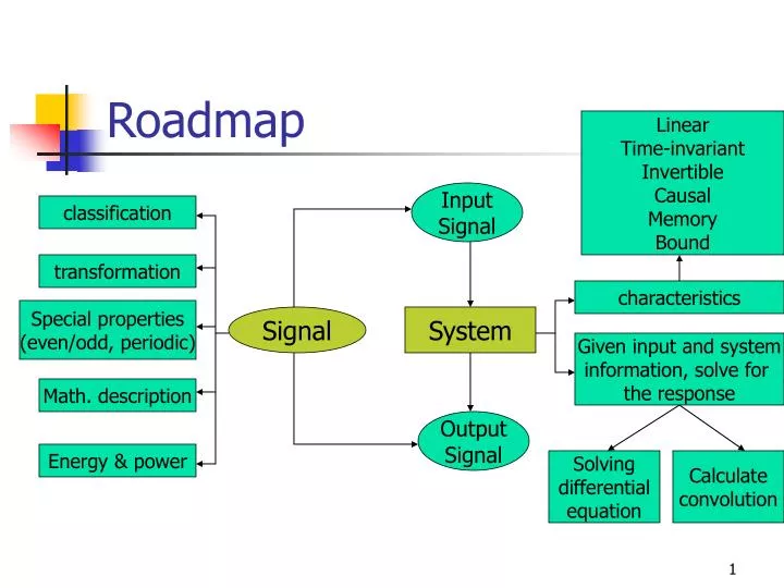
1. Roadmap Linear Time-invariant Invertible Causal Memory Bound Input Signal classification transformation characteristics Special properties (even/odd, periodic) Signal System Given input and system information, solve for the response Math. description Output Signal Energy & power Solving differential equation Calculate convolution

2. ECE310 – Lecture 13 Fourier Series - CTFS 02/26/01

3. Why a New Domain? • It is often much easier to analyze signals and systems when they are represented in the frequency domain • The entire subject of signals & systems consists primarily the following concepts: • Writing signals as functions of frequency • Looking at how systems respond to inputs of different frequencies • Developing tools for switching between time-domain and frequency-domain representations • Learning how to determine which domain is best suited for a particular problem

4. Scenario for Selected Legs

5. two legs selected

6. two legs selected

7. Leg1 Analysis (AAV from N to W)

8. Leg1 Analysis (DW from W to E)

9. Fourier Series & Fourier Transform • They both represent signal in the form of a linear combination of complex sinusoids • FS can only represent periodic signals for all time • FT can represent both periodic and aperiodic signals for all time

10. Limitations of FS • Dirichlet conditions • The signal must be absolutely integrable over the time, t0 < t < t0 + TF • The signal must have a finite number of maxima and minima in the time, t0 < t < t0 + TF • The signal must have a finite number of discontinuities, all of finite size in the time, t0 < t < t0 + TF

11. The Fourier Series of x(t) over TF • Fourier series (xF) represents any function over a finite interval TF • Outside TF, xF repeats itself periodically with period TF. • xF is one period of a periodic function which matches the function x(t) over the interval TF. • If x(t) is periodic with period = T0 • if TF=nT0, then the Fourier series representation (TSR) equals to x(t) everywhere; • if TF != nT0, then FSR equals to s(t) only in the time period TF, not anywhere else.

12. Examples

13. The Fourier Series

14. Some Parameters • TF is the interval of signal x(t) over which the Fourier series represents • fF = 1/TF is the fundamental frequency of the Fourier series representation • n is called the “harmonic number” • 2fF is the second harmonic of the fundamental frequency fF. • The Fourier series representation is always periodic and is linear combinations of sinusoids at fF and its harmonics.

15. Interpretation • The FS coefficient tells us how much of a sinusoid at the nth harmonic of fF are in the signal x(t) • In another word, how much of one signal is contained within another signal

16. Calculation of FS • Sinusoidal signal (ex 1,2) • Non-sinusoidal signal (ex 3) • Periodic signal over a non-integer number of periods (ex 4) • Periodic signal over an integer number of periods (ex 4) • Even and odd periodic signals (ex 5) • Random signal (no known mathematical description) (ex 6)

17. Example 1 – Finite Nonzero Coef • x(t) = 2cos(400pt) over 0<t<10ms • Band-limited signals • Analytically • Trignometric form and Complex form • Graphically (p6-10~6-12)

18. Example 2 – Finite Nonzero Coef • x(t) = 0.5 - 0.75cos(20pt) + 0.5sin(30pt) over -100ms < t < 100ms • Band-limited signals (p6-14,6-15)

19. Example 3 – Infinite Nonzero Coef • x(t) = rect(2t)*comb(t) over –0.5<t<0.5 • When we have infinite nonzero coefficients, we tend to use magnitude and phase of the CTFS versus harmonic to present the CTFS (p6-19)

20. Example 4 – Periodic Signal • x(t) = 2cos(400pt) over 0<t<7.5ms • Over a non-integer number of period • p6-20

21. Example 5 – Periodic Even/Odd Signals • For a periodic even function, X[k] must be real and Xs[k] must be zero for all k • For a periodic odd function, X[k] must be imaginary and Xc[k] must be zero for all k

22. Example 6 – Random Signal • Is it necessary to know the mathematical description of the signal in order to derive its CTFS? • No • Graphically (p6-24, 6-25)

23. Convergence of the CTFS • For continuous signal • As N increases, CTFS approaches x(t) in that interval • For signals with discontinuities • As N increases, there is an overshoot or ripple near the discontinuities which does not decrease – Gibbs phenomenon • When N goes to infinity, the height of the overshoot is constant but its width approaches zero, which does not contribute to the average power

24. Example • P6-35, 6-36

25. Exercises 6.1.2

26. Response of LTI System with Periodic Excitation • Represent the periodic excitation using complex CTFS • Since it’s an LTI system, the response can be found by finding the response to each complex sinusoid • Example: RC lowpass circuit • Magnitude and phase of Vout[k]/Vin[k] (p6-53)

27. Properties of CTFS • Linearity • Time shifting • Time reversal • Time scaling • Time differentiation • Time integration • Time multiplication • Frequency shifting • Conjugation • Parseval’s theorem

28. Parseval’s Theorem • Only if the signal is periodic • The average power of a periodic signal is the sum of the average powers in its harmonic components

29. Summary - CTFS • The essence of CTFS • The limitation of CTFS • The calculation of CTFS • The convergence of CTFS • Continuous signals • Signals with discontinuities – Gibbs phenomena • Properties of CTFS • Especially Parseval’s theorem • Application in LTI system

30. Test 2