Download
1 / 23
250 likes | 463 Views
p. e +. 0. . e -. +. Atmospheric Neutrinos. +. Phenomenology and Detection. . Michelangelo D’Agostino Physics C228 October 18, 2004. Outline. Cosmic Rays and Atmospheric Generation Flavor Oscillations Cerenkov Radiation SuperKamiokande SNO AMANDA/IceCube.

E N D
p e+ 0 e- + Atmospheric Neutrinos + Phenomenology and Detection Michelangelo D’Agostino Physics C228 October 18, 2004
Outline • Cosmic Rays and Atmospheric Generation • Flavor Oscillations • Cerenkov Radiation • SuperKamiokande • SNO • AMANDA/IceCube
Cosmic Rays • Earth is constantly bombarded by a stream of charged particles • 86% protons • 11% alpha particles • 1% heavier elements up to uranium • 2% electrons • Except for the highest energy constituents, they’re galactic in origin
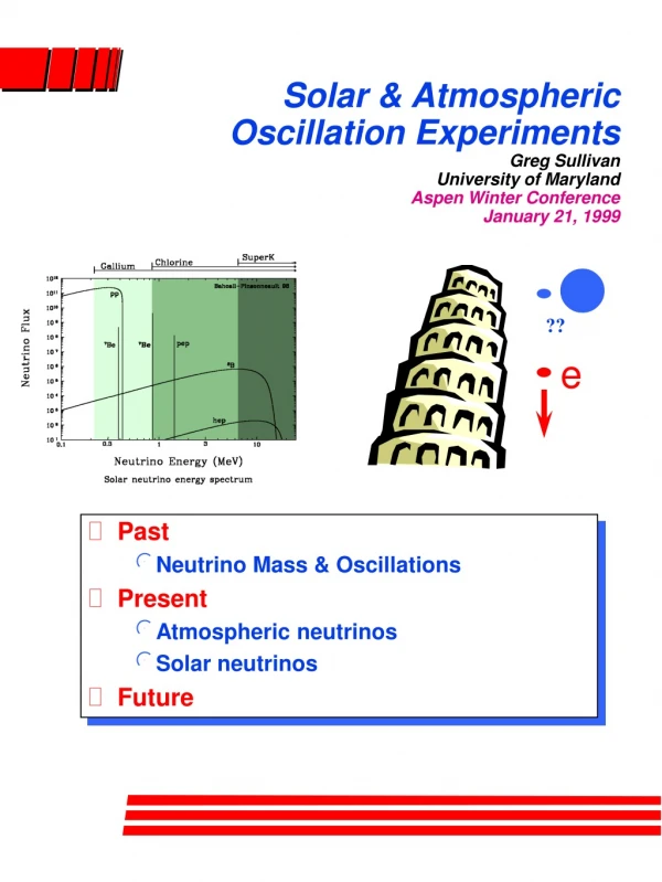
Cosmic Rays • The flux follows an E-2.7 distribution up to knee • E-3.0 after • spectrum shows an ankle • Controversy over highest energy cosmic rays, above ~1020 eV • would have to come from our local cluster because of the so-called GZK effect unknown acceleration mechanism Knee Knee Knee Ankle Ankle Ankle F. Halzen
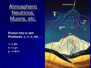
Cosmic Rays • These primary cosmic ray particles slam into the atmosphere and generate secondary mesons • Most commonly produced particles are pions +,-,0 and kaons • below 100 GeV the ’s decay before interacting ++ + -- + • 02e+e- cascades hard component soft component
Cosmic Rays • ’s from the hard component further decay to neutrinos via - e- +e + and the conjugate decay for + • energy spectrum peaks at around .25 GeV and falls off as E-2.7 at higher energies • we get one produced from pion decay into the plus a e and from the decay, so we’d roughly expect a 2:1 ratio of atmospheric to e generated by cosmic rays in the atmosphere
ratio 2 Cosmic Rays Ref. 2 above a few GeV, up-going and down-going fluxes are symmetric; this is an important observation for oscillation experiments is the zenith angle, so cos =-1 is an up-going (through the Earth) while cos =-1 is down-going
Flavor Oscillations • in the 1980’s, underground detectors set up to look for proton decay found that the atmospheric flux reaching the ground did not have the expected flavor ratio • this suggested that the ’s might be changing their flavor while traveling through the atmosphere • solar investigations found that e’s could oscillate; it now appeared that ’s could oscillate as well • atmospheric studies were ideal because one could vary the two important parameters, path length by looking at different zenith angles and energy by looking at different neutrino energies
Flavor Oscillations • the basic idea is that ’s are created as eigenstates of flavor, but that they propagate as eigenstates of mass • for two state mixing, the two sets of states are connected via where is the mixing angle • is some linear combination of the 1, 2 mass eigenstates; each of these eigenstates develops in time with the usual factor of where
Flavor Oscillations • we tack this factor onto each i and use t=L/c, where L is the distance traveled, and then compute the probability of observing • there is a finite probability that will oscillate into • the MSW effect, which describes oscillations in matter and is crucial important for solar neutrino oscillations, only needs to be considered for oscillations involving e, so we don’t need to consider it here
Cerenkov Radiation • Cerenkov Radiation is the primary means used to detect these ’s • when a charged particle moves through a medium at a speed greater than the speed of light in the medium, it emits Cerenkov photons wavefront so particle or
this is analogous to a sonic boom timing of photons allows for reconstruction of the path of the charged particle Cerenkov Radiation F. Halzen
SuperK • 50,000 tons of water densely instrumented with 11,000 photo- multiplier tubes • Cerenkov cone intersects water surface, forming a ring • timing of pulses can be used to reconstruct direction • e- and - give different rings; e- is more diffuse due to multiple scattering
SuperK - e- Ref. 1
SNO • 1,000 tons of heavy water, D2O, surrounded by ultrapure water to shield out radioactivity • 9,500 PMT’s
SuperK-Results The results for electron neutrinos agreed with expectations, but for muon neutrinos there was a clear deficit. Furthermore, it depended on distance traveled (as up-going muon neutrinos showed a larger deficit), and it depended on energy (the upper trace, lower energy, shows a greater deficit for all distances). The interpretation is that muon neutrinos oscillate into tau neutrinos. e Ref. 2 up-going, L13,000 km down-going, L15 km
SuperK-Results Ref. 1 The quantity Aencapsulates the asymmetry. Without oscillations, we expectA=0. The observationdeviates from A=0 by 7.5 Observed /e over Monte Carlo /e for various experiments.
SuperK-Results Ref. 3 sinusoidal dependence in L/E that can’t be explained by Monte Carlo without oscillations
SuperK-Results Ref. 3 Results are traditionally plotted as contours in them2, sin22 plane where m2 is the mass difference andsin22 is the mixing angle. 1.9x10⁻³<m2<3.0x10⁻³ eV2 sin22>.90
50 m AMANDA/IceCube • Embedded in the South Polar ice cap, AMANDA and IceCube are large-scale, more sparsely instrumented detectors with higher energy thresholds SuperK • intended to look for ’s of extraterrestrial origin, e.g. from gamma ray bursts, supernovae, active galactic nuclei, decays of dark matter particles • atmospheric ’s are a background nuisance; not really sensitive to oscillations
South Pole AMANDA– 1 mile deep F. Halzen
References For a basic introduction to cosmic rays and oscillations, see Donald Perkins, Particle Astrophysics. [1] T. Kajita and Y. Totsuka. “Observation of atmospheric neutrinos.” Rev. Mod. Phys. 73, 85. 2001. [2] M.C. Gonzalez-Garcia and Y. Nir. “Neutrino masses and mixing: evidence and implications.” Rev. Mod. Phys. 75, 345. 2003. [3] Y. Ashie et al. “Evidence for an Oscillatory Signature in Atmospheric Neutrino Oscillations.” Phys. Rev. Lett. 93, 101801-1. 2004.