Download

1 / 45
450 likes | 623 Views
Probability Review. Georgios Varsamopoulos School of Computing and Informatics Arizona State University. Problem 1. We roll a regular dice and we toss a coin as many times as the roll indicates. What is the probability that we get no tails? What is the probability that we get 3 heads?

E N D
Probability Review Georgios VarsamopoulosSchool of Computing and InformaticsArizona State University
Problem 1 • We roll a regular dice and we toss a coin as many times as the roll indicates. • What is the probability that we get no tails? • What is the probability that we get 3 heads? • Using the same process, we are asked to get at least 6 tails in total. • If we don’t get 6 tails with the first roll, we roll again and repeat as many times as needed to get at least 6 tails. • What is the probability that we need more than 1 rolls to get 6 tails?
Problem 2 • A process has to send 1000 bytes over a wireless link using a stop-and-wait protocol. The payload size per packet is 10 bytes. The bit-wise error probability is 10-3. • Find the expected number of total packet transmissions needed to transfer the 1000 bytes.
The Markov Process • Discrete time Markov Chain: is a process that changes states at discrete times (steps). Each change in the state is an event. • The probability of the next state depends solely on the current state, and not on any of the past states: • Markov Process’s versatility • can be used in building mobility models, data traffic models, call pattern models etc.
Transition Matrix • Putting all the transition probabilities together, we get a transition probability matrix: • The sum of probabilities across each row has to be 1.
Stationary Probabilities • We denote Pn,n+1 as P(n). If for each step n the transition probability matrix does not change, then we denote all matrices P(n) as P. • The transition probabilities after 2 steps are given by PP=P2; transition probabilities after 3 steps by P3, etc. • Usually, limnPn exists, and shows the probabilities of being in a state after a really long period of time. • Stationary probabilities are independent of the initial state
Numeric Example • No matter where you start, after a long period of time, the probability of being in a state will not depend on your initial state.
r r r 1 1 q q q 1 2 3 4 5 p p p Markov Random Walk • A Random Walk Is a subcase of Markov chains. • The transition probabilitymatrix looks like this:
Markov Random Walk • Hitting probability (gambler’s ruin) ui=Pr{XT=0|Xo=i} • Mean hitting time (soujourn time) vi=E[T|Xo=k]
A D Example Problem • A mouse walks equally likely between adjacent rooms in the following maze: • Once it reaches room D, it finds food and stays there indefinitely. • What is the probability that it reaches room D within 5 steps, starting in A? • Is there a probability it will never reach room D?
0.01 0.99 LOW HIGH 0.9 0.1 Example Problem 2 • A variable bit rate (VBR) audio stream follows a bursty traffic model described by the following two-state Markov chain: • In the LOW state it has a CBR of 50Kbps and in the HIGH it has a CBR of 150Kbps. • What is the average bit-rate of the stream?
Example Problem 2 (cont’d) • We find the stationary probabilities • Using the stationary probabilities we find the average bitrate:
Continuous time Markov chains • Simple variation of the time-discrete markov chain • Self-transitions, i.e. (n,n) transitions, are replaced with the PDF of the pause. • At any state, the process remains for a random time under exponential distribution
Mobility Models for Mobile Computing Georgios VarsamopoulosSchool of Computing and InformaticsArizona State University
Mobility models play an important role in various layers Location management Routing Location-aware applications Mobility models are used in three phases in developing a LM scheme At assumptions phase At performance analysis phase At simulation phase Analytical vs simulation mobility models two types of mobility models: Aggregate (analytical) per-user (simulation) Two granularity domains of mobility models: Discrete space Continuous space Aggregate mobility models flow models per-user mobility models based on a stochastic modeling of velocity. random way-point (RWP) Angular RWP Habitual models Trip-based mobility model Markovian models Variations Time-dependent behavior (temporal dependency) Location-dependent behavior (spatial dependency) Mobility models
Random Waypoint Process (WRP) • First appeared in the publication of DSR[1996] • Basic configuration • Choose a random target point (waypoint) distributed (usually uniformly) over some area • Move from current location to the target waypoint using a constant velocity 0 2 vo vo vo 1 3
RWP variants/extensions • Non-uniform distribution of waypoint selection • Uniform distribution makes the nodes spend more time around the center • Pause times • Select a random or a constant time to wait at each destination • Random velocities • Choose a random velocity and move from current location to the target waypoint using this velocity 0 2 vo v1 v2 1 3
Random Turn Process • Choose a random direction (way) distributed (usually uniformly) over [0, 2π] • Choose a random velocity and move from current location over specified direction for certain time or distance. 0 1 2 v1 3 v2 2 v3 1 3
Markovian:Random Graph Mobility Process • A random walk mobility model Gu for a user u: • Nodes represent regions • Weighted directed edge • an edge r1-> r2 has weight: Pr[ user will mover to r2 when it leaves r1] • Pr[path p in Gu] = product of probabilities of all edges in p. • In general, Gu has cycles
P(n,m)(n,m+1) P(n,m)(n+1,m) Grid-based markovian mobility model(2-d random walk) • Based on a time-continuous, space-discrete 2-D markov chain • Can be used to model urban mobility
P(n,m)(n,m+1) Hex-based markovian mobility model • Variation of the 2-d model • Can be used in cellular systems
Probability Review Georgios VarsamopoulosSchool of Computing and InformaticsArizona State University
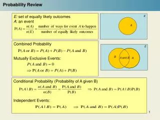
Basic concepts and terminology • Basic concepts by example: dice rolling • (Intuitively) coin tossing and dice rolling are Stochastic Processes • The outcome of a dice rolling is an Event • The values of the outcomes can be expressed as a Random Variable, which assumes a new value with each event. • The likelihood of an event (or instance) of a random variable is expressed as a real number in [0,1]. • Dice: Random variable • instances or values: 1,2,3,4,5,6 • Events: Dice=1, Dice=2, Dice=3, Dice=4, Dice=5, Dice=6 • Pr{Dice=1}=0.1666 • Pr{Dice=2}=0.1666 • The outcome of the dice is independent of any previous rolls (given that the constitution of the dice is not altered)
Basic Probability Properties • The sum of probabilities of all possible values of a random variable is exactly 1. • Pr{Coin=HEADS}+Pr{Coin=TAILS} = 1 • The probability of the union of two events of the same variable is the sum of the separate probabilities of the events • Pr{ Dice=1 Dice=2 } = Pr{Dice=1}+{Dice=2} = 1/3
Properties of two or more random variables • The tossing of two or more coins (such that each does not touch any of the other(s) ) simulateously is called (statistically) independent processes (so are the related variables and events). • The probability of the intersection of two or more independent events is the product of the separate probabilities: • Pr{ Coin1=HEADS Coin2=HEADS } =Pr{ Coin1=HEADS} Pr{Coin2=HEADS}
Conditional Probabilities • The likelihood of an event can change if the knowledge and occurrence of another event exists. • Notation: • Usually we use conditional probabilities like this:
Conditional Probability Example • Problem statement (Dice picking): • There are 3 identical sacks with colored dice. Sack A has 1 red and 4 green dice, sack B has 2 red and 3 green dice and sack C has 3 red and 2 green dice. We choose 1 sack equally randomly and pull a dice while blind-folded. What is the probability that we chose a red dice? • Thinking: • If we pick sack A, there is 0.2 probability that we get a red dice • If we pick sack B, there is 0.4 probability that we get a red dice • If we pick sack C, there is 0.6 probability that we get a red dice • For each sack, there is 0.333 probability that we choose that sack • Result ( R stands for “picking red”):
Moments and expected values • mth moment: • Expected value is the 1st moment: X =E[X] • mth central moment: • 2nd central moment is called variance (Var[X],2X)
Geometric Distribution • Based on random variables that can have 2 outcomes (A and A): Pr{A}, Pr{A}=1-Pr{A} • Expresses the probability of number of trials needed to obtain the event A. • Example: what is the probability that we need k dice rolls in order to obtain a 6? • Formula: (for the dice example, p=1/6)
Geometric distribution example • A wireless network protocol uses a stop-and-wait transmission policy. Each packet has a probability pE of being corrupted or lost. • What is the probability that the protocol will need 3 transmissions to send a packet successfully? • Solution: 3 transmissions is 2 failures and 1 success, therefore: • What is the average number of transmissions needed per packet?
Binomial Distribution • Expresses the probability of some events occurring out of a larger set of events • Example: we roll the dice n times. What is the probability that we get k 6’s? • Formula: (for the dice example, p=1/6)
Binomial Distribution Example • Every packet has n bits. There is a probability pΒthat a bit gets corrupted. • What is the probability that a packet has exactly 1 corrupted bit? • What is the probability that a packet is not corrupted? • What is the probability that a packet is corrupted?
Continuous Distributions • Continuous Distributions have: • Probability Density function • Probability Distribution function:
Continuous Distributions • Normal Distribution: • Uniform Distribution: • Exponential Distribution:
Poisson Distribution • Poisson Distribution is the limit of Binomial when n and p 0, while the product np is constant. In such a case, assessing or using the probability of a specific event makes little sense, yet it makes sense to use the “rate” of occurrence (λ=np). • Example: if the average number of falling stars observed every night is λ then what is the probability that we observe k stars fall in a night? • Formula:
Poisson Distribution Example • In a bank branch, a rechargeable Bluetooth device sends a “ping” packet to a computer every time a customer enters the door. • Customers arrive with Poisson distribution of customers per day. • The Bluetooth device has a battery capacity of m Joules. Every packet takes n Joules, therefore the device can send u=m/n packets before it runs out of battery. • Assuming that the device starts fully charged in the morning, what is the probability that it runs out of energy by the end of the day?
Poisson Process • It is an extension to the Poisson distribution in time • It expresses the number of events in a period of time given the rate of occurrence. • Formula • A Poisson process with parameter has expected value and variance . • The time intervals between two events of a Poisson process have an exponential distribution (with mean 1/).
Poisson dist. example problem • An interrupt service unit takes to sec to service an interrupt before it can accept a new one. Interrupt arrivals follow a Poisson process with an average of interrupts/sec. • What is the probability that an interrupt is lost? • An interrupt is lost if 2 or more interrupts arrive within a period of to sec.