Download
1 / 46
460 likes | 578 Views
Intermediate disturbance and ant communities in a forested ecosystem. John H. Graham, Anthony J. . Krzysik, Dave A. Kovacic, D. Carl Freeman, W. Russell Long, Jonathan Nutter, Jeffrey J. Duda, John M. Emlen, John C. Zak, Mike Wallace, Catherine Chamberlin-Graham, and Hal Balbach.

E N D
Intermediate disturbance and ant communities in a forested ecosystem John H. Graham, Anthony J.. Krzysik, Dave A. Kovacic, D. Carl Freeman, W. Russell Long, Jonathan Nutter, Jeffrey J. Duda, John M. Emlen, John C. Zak, Mike Wallace, Catherine Chamberlin-Graham, and Hal Balbach
Intermediate-Disturbance Hypothesis from Connell (1978)
Intermediate-DisturbanceHypothesis • Intensity of disturbance (mild to intense) • Frequency of disturbance (infrequent to frequent) • Scale of disturbance (small to large) • Duration of disturbance (brief to continuous)
Examples of Intermediate Disturbance Coral-reef communities Courtesy of Bill Davin
Tropical rain forest communities Courtesy of Marty Cipollini
Does arthropod diversity fit the intermediate disturbance hypothesis? • Some studies support IDH • Gallé 1991 • Szentkiralyi and Kozar 1991 • Young et al. 1997) • Some studies do not support IDH • Greenslade and Greenslade 1977 • Járdán et al. 1993 • Rambo and Faeth 1999 • Floren et al. 2001)
Ants possess the three criteria necessary for a hump-backed species diversity curve:(Fuentes and Jaksić 1988) • disturbance substantially reduces their abundance • propagules (winged queens) are available for colonization • colonizing species compete strongly (most colonies have a regular spatial distribution). Dorymyrmex bureni
Site Classification • 40 sites were classified on a scale from 1-10 based on a visual assessment of the level of disturbance where: 1 10 Low Disturbance Highly Disturbed
Disturbance Class Sand and Clay A Horizon Depth Soil Compaction Canopy Cover Max. Basal Area Avg. Basal Area Tree Density Bare Ground Forb Cover Grass Cover Woody Cover Pine Seedlings Total Ground Cover Years Since Last Fire Fire Frequency Environmental Variables
Collection Method Pitfall Traps
Site E5. Disturbance class 1, D = 5.26.Mesic deciduous forest (oak-hickory). Five species of ants.
Site A15. Disturbance class 2, D = 16.01. Longleaf pine. Seven species of ants.
Site D3-1. Disturbance class 4, D = 34.9. Mixed pine-oak-hickory. Twenty one species of ants.
Site D15-4. Disturbance class 7; D = 49.68. Mixed pine and oak. Twenty five species of ants.
Site D6-1. Disturbance class 9; D = 83.66. Mixed pine-oak. Eight species of ants.
Site D15-1. Disturbance class 10; D = 100. Mixed pine-oak. Four species of ants.
Hypotheses • Storage effect (Chesson 1981) • Spatial heterogeneity (MacArthur and MacArthur 1961) • Net primary productivity (Margalef 1963, Grime 1973)
Storage-effect hypothesis • Trade-offs between competition and dispersal • Disturbance reduces the density of competitive species having poor dispersal, thereby creating opportunities for less competitive ones having good dispersal • With intermediate disturbance, both competitive and weedy species co-exist
Predictions of the storage-effect hypothesis • Spatial or temporal variation in habitat quality • Trade off between dispersal and competition (r- and K-selected species)
r- and k- Selection in Ants • r-selected species • large colonies • small workers • poor competitors • k-selected species • small colonies • large workers • good competitors Holldobler and Wilson (1990)
Canonical Correspondence Analysis Environmental Vectors
Canonical Correspondence Species Scores
Species associated with high disturbance: Pogonomyrmex badius Dorymyrmex smithi Pheidole bicarinata
No support for the storage-effect hypothesis • Colony size is unrelated to disturbance (independent contrasts, r = 0.421, n = 10, P > 0.05) • Worker size is unrelated to disturbance (r = -0.009, n = 46, P > 0.95) • Ability to defend a bait is unrelated to disturbance (independent contrasts, r = -0.111, n = 13, P > 0.05)
Worker size (PC1) versus location on the disturbance gradient (CCA1)
Spatial-heterogeneity hypothesis • Increased spatial heterogeneity in moderately disturbed landscapes • Encourages niche diversification • Greater numbers of co-existing species
Predictions of Spatial Heterogeneity Hypothesis • Spatial heterogeneity should be greatest for intermediate disturbance • Species diversity should be correlated with spatial heterogeneity
r2 = 0.454 P < 0.001
r = 0.419 P < 0.05
Predictions of Net Primary Productivity Hypothesis • Net Primary Productivity should be greatest for intermediate disturbance • Species diversity should be correlated with Net Primary Productivity
Normalized difference vegetation index (NDVI) • Measures the “greenness” of vegetation • Strongly correlated with standing crop • Correlated with net primary productivity
r = 0.820 P < 0.0001
Deforestation increases soil temperature • Ants like warm habitats • Undisturbed, but productive, forest may be too cool for many species of ants • Cool temperatures may interfere with the ability of ants to accumulate resources
Predicted maximum daily temperature Disturbance and Soil Surface Temperature
Date that soil temperature first exceeded 25 degrees Celsius versus canopy cover r = 0.916 P < 0.05
Available NPP • Because ant activity is tied to temperature, we developed a measure of available net primary production • We define available NPP as the product of NDVI and the estimated number of days the maximum soil temperature exceeded 25 degrees C
r = 0.394 P < 0.05
Conclusions • Species richness is highest for intermediate levels of disturbance and intermediate NDVI • Spatial heterogeneity is greatest in moderately disturbed sites • Species richness is linearly related to spatial heterogeneity • Species richness is linearly related to the product of NDVI and the number of days maximum soil temperature exceeded 25 degrees C (available NPP) • Species richness is not related to predictions of the storage-effect hypothesis