Download
1 / 51
530 likes | 792 Views
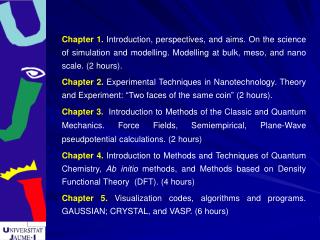
Chapter 1. Introduction, perspectives, and aims. On the science of simulation and modelling. Modelling at bulk, meso, and nano scale. (2 hours). Chapter 2. Experimental Techniques in Nanotechnology. Theory and Experiment: “Two faces of the same coin” (2 hours).

E N D
Chapter 1. Introduction, perspectives, and aims. On the science of simulation and modelling. Modelling at bulk, meso, and nano scale. (2 hours). Chapter 2. Experimental Techniques in Nanotechnology. Theory and Experiment: “Two faces of the same coin” (2 hours). Chapter 3. Introduction to Methods of the Classic and Quantum Mechanics. Force Fields, Semiempirical, Plane-Wave pseudopotential calculations. (2 hours) Chapter 4. Introduction to Methods and Techniques of Quantum Chemistry, Ab initio methods, and Methods based on Density Functional Theory (DFT). (4 hours) Chapter 5. Visualization codes, algorithms and programs. GAUSSIAN; CRYSTAL, and VASP. (6 hours)
. Chapter 6. Calculation of physical and chemical properties of nanomaterials. (2 hours). Chapter 7. Calculation of optical properties. Photoluminescence. (3 hours). Chapter 8. Modelization of the growth mechanism of nanomaterials. Surface Energy and Wullf architecture (3 hours) Chapter 9. Heterostructures Modeling. Simple and complex metal oxides. (2 hours) Chapter 10. Modelization of chemical reaction at surfaces. Heterogeneous catalysis. Towards an undertanding of the Nanocatalysis. (4 hours)
Chapter 5.Visualization codes, algorithms and programs Lourdes Gracia y Juan Andrés Departamento de Química-Física y Analítica Universitat Jaume I Spain & CMDCM, Sao Carlos Brazil Sao Carlos, Novembro 2010
PROGRAM Graphical Interface XCrysDen, Jmol Ana-Band-DOS - CRYSTAL Molden - VASP GaussView - GAUSSIAN
CRYSTAL CRYSTAL performs ab initio calculations on periodic systems within the linear combination of atomic orbitals (LCAO) approximation. That is, the crystalline orbitals (CO) are treated as linear combinations of Bloch functions (BF), defined in terms of local functions, hereafter indicated as atomic orbitals (AO). Those local functions are expressed as linear combination of a certain number of Gaussian type functions (GTF). The "CRYSTAL tutorial project" : http://www.theochem.unito.it/crystal_tuto/mssc2008_cd/tutorials/index.html
GEOMETRY - The bulk structure (conventional cell, primitive cell) - Creating a super cell - Symmetry and geometry editing - Removal, addition, substitution, displacement of atoms - 2D input; the slab model input keywords ATOMSUBS substitution of atoms ATOMREMO removal of atoms ATOMINSE addition of atoms ATOMDISP displacement of atoms ATOMROT rotation of groups of atoms SUPERCEL generation of super cell SLABCUT generation of a slab parallel to a given plane
SLABCUT generation of a slab parallel to a given plane Planes with different Miller indices in cubic crystals (ℓmn) denotes a plane that intercepts the three points a1/ℓ, a2/m, and a3/n
Basis set http://www.crystal.unito.it/Basis_Sets/Ptable.html ECPs The idea behind pseudopotentials is to treat the core electrons as effective averaged potentials rather than actual particles. Thus, pseudopotentials are modifications to the Hamiltonian.
Density Functional Theory (DFT) methods The keyword DFT selects a DFT Hamiltonian. Exchange-correlation functionals are separated in an exchange component (keyword EXCHANGE) and a correlation component (keyword CORRELAT). Hybrid: the exchange functional is a linear combination of Hartree-Fock, local and gradient-corrected exchange term B3PW B3LYP EXCHANGE EXCHANGE BECKE BECKE CORRELAT CORRELAT PWGGA LYP HYBRID HYBRID 20 20 NONLOCAL NONLOCAL 0.9 0.81 0.9 0.81 % of Hartree-Fock exchange weight of non local exchange and correlation
EXAMPLE A PZT ten-layer slab model of the PT(100) surface. Substitution:40%Zr and 60% Ti PZT-4060 CRYSTAL 0 0 0 99 4.017 4.14 4 282 0.0 0.0 -0.029665 8 -0.5 -0.5 0.126996 8 0.0 -0.5 -0.373995 22 -0.5 -0.5 -0.479824 SLABCUT 1 0 0 1 10 ATOMSUBS 2 3 40 23 40 OPTGEOM ENDOPT ENDG 282 2 DURAND 0 1 3 2.0 1.0 0 1 1 2.0 1.0 22 7 0 0 8 2. 1. 0 1 6 8. 1. 0 1 4 8. 1. 0 1 1 2.0 1.0 0 1 1 0.0 1.0 0 3 4 2.0 0.972 0 3 1 0.0 1.0 8 4 0 0 6 2.0 1.0 0 1 3 6.0 1.0 0 1 1 0.0 1.0 0 3 1 0.0 1.0 40 8 0 0 9 2. 1. 0 1 7 8. 1. 0 1 6 8. 1. 0 1 3 8. 1. 0 3 6 10. 1. 0 1 1 2. 1. 0 3 2 2. 1. 0 3 1 0. 1. 99 0 END DFT B3LYP END SCFDIR TOLINTEG 8 8 8 8 14 SHRINK 4 4 LEVSHIFT 3 1 MAXCYCLE 100 FMIXING 30 END P 4 M M slab model ten layers substitution Hybrid functional pseudopotential Coulomb and Exchange series tolerances Pack-Monkhorst and Gilat shrinking factors level shifter used to help convergence % of hamiltonian matrix mixing to help convergence
OUTPUT ZrO2 PbO TiO2 PbO TiO2 PbO TiO2 PbO ZrO2 PbO ************************************************************************************ LATTICE PARAMETERS (ANGSTROMS AND DEGREES) - BOHR = 0.5291772083 ANGSTROM PRIMITIVE CELL A B C ALPHA BETA GAMMA 4.01700000 4.14000000 500.00000000 90.000000 90.000000 90.000000 ******************************************************************************* ATOMS IN THE ASYMMETRIC UNIT 25 - ATOMS IN THE UNIT CELL: 25 ATOM X/A Y/B Z(ANGSTROM) ******************************************************************************* 1 T 8 O -5.000000000000E-01 1.269960000000E-01 9.038250000000E+00 2 T 8 O 0.000000000000E+00 -3.739950000000E-01 9.038250000000E+00 3 T 40 ZR -5.000000000000E-01 -4.798240000000E-01 9.038250000000E+00 4 T 282 PB 0.000000000000E+00 -2.966500000000E-02 7.029750000000E+00 5 T 8 O -5.000000000000E-01 -3.739950000000E-01 7.029750000000E+00 6 T 8 O -5.000000000000E-01 1.269960000000E-01 5.021250000000E+00 7 T 8 O 0.000000000000E+00 -3.739950000000E-01 5.021250000000E+00 8 T 22 TI -5.000000000000E-01 -4.798240000000E-01 5.021250000000E+00 9 T 282 PB 0.000000000000E+00 -2.966500000000E-02 3.012750000000E+00 10 T 8 O -5.000000000000E-01 -3.739950000000E-01 3.012750000000E+00 11 T 8 O -5.000000000000E-01 1.269960000000E-01 1.004250000000E+00 12 T 8 O 0.000000000000E+00 -3.739950000000E-01 1.004250000000E+00 13 T 22 TI -5.000000000000E-01 -4.798240000000E-01 1.004250000000E+00 14 T 282 PB 0.000000000000E+00 -2.966500000000E-02 -1.004250000000E+00 15 T 8 O -5.000000000000E-01 -3.739950000000E-01 -1.004250000000E+00 16 T 8 O -5.000000000000E-01 1.269960000000E-01 -3.012750000000E+00 17 T 8 O 0.000000000000E+00 -3.739950000000E-01 -3.012750000000E+00 18 T 22 T I -5.000000000000E-01 -4.798240000000E-01 -3.012750000000E+00 19 T 282 PB 0.000000000000E+00 -2.966500000000E-02 -5.021250000000E+00 20 T 8 O -5.000000000000E-01 -3.739950000000E-01 -5.021250000000E+00 21 T 8 O -5.000000000000E-01 1.269960000000E-01 -7.029750000000E+00 22 T 8 O 0.000000000000E+00 -3.739950000000E-01 -7.029750000000E+00 23 T 40 ZR -5.000000000000E-01 -4.798240000000E-01 -7.029750000000E+00 24 T 282 PB 0.000000000000E+00 -2.966500000000E-02 -9.038250000000E+00 25 T 8 O -5.000000000000E-01 -3.739950000000E-01 -9.038250000000E+00
Spin-polarized systems an unrestricted calculation must be performed - UHF in input block 3 for HF hamiltonian - SPIN in DFT input block for DFT hamiltonian preparing an SCF guess driving the system to the desired spin state. input keywords DFT B3LYP SPIN END … SPINLOCK2 2000 ATOMSPIN 2 1 1 2 1 lock in a given spin state alpha-beta electrons locked to 2 for 2000 scf cycles atom 1 and 2 have formally the same spin in the atomic wave function
Anti ferromagnetic phase - 2 electrons up, 2 electrons down, total spin 0 NiO – CRYSTAL 0 1 1 225 4.164 2 28 0. 0. 0. 8 .5 .5 .5 SUPERCEL 0 1 1 1 0 1 1 1 0 END basis set input END UHF TOLINTEG 7 7 7 7 14 END 8 8 TOLENE 7 LEVSHIFT 3 1 SPINLOCK 0 50 ATOMSPIN 2 1 1 2 -1 MAXCYCLE 90 END Example: antiferromagnetic phase (NiO) Pack-Monkhorst and Gilat shrinking factors 2 Nickel atoms with antiparallel spins. Total spin 0 atom 1 and 2 have formally opposite spin in the atomic wavefunction
output Frequency calculation input
Vibrational frequencies Jmol interface http://www.theochem.unito.it/crystal_tuto/mssc2008_cd/jmoledit/index.html
input Frequency calculation output
Here are the total atomic charges obtained at different level of theory: Note that Mulliken population analysis is an arbitrary scheme for partitioning total electron charge in atom and bond contributions. Atomic charges, unlike the electron density, are not a quantum mechanical observable, and are not unambiguously predictable from first principles. Electron properties • Atoms and bond populations (Mulliken scheme) • Electron Charge Density • Band Structure • Density of States PPAN XCrysDen ECHG BAND ANA-BAND-DOS DOSS
Input ECHG ECHG 0 65 COORDINA -4. -4. 0.0 4. -4. 0.0 4. 4. 0.0 END Nº of point along the B-A segment ECHG → XCrysDen CRYSTAL computes the charge density in a grid of points defined in input. -total electron density maps -difference maps: difference between the crystal electron density and a "reference" electron density.
ECHG → XCrysDen Example: Slab PZT
ECHG → XCrysDen Example: Bulk ST Supercell 2x2x2
Band Structure: ANA-BAND by Nélio H. Nicoleti, POSMAT, Campus Bauru Input Band
Fermi energy (eV) -points
8 6 4 2 E (eV) 0 -2 -4 -6 k1 k2 k3 k4 k5 Fermi energy (-4.04 eV) scaled at 0
Density of States: ANA-DOS R points of .out Only T of .out
Input: DOS total Density of States: ANA-DOS Output: DOS projection onto all the AOs
dxy Input: DOS atomico dxz dy 2 dz 2 dx - y 2 2 .inf from ANA-DOS .inf
Pb O Ti tot dxy dy2 dz2 dx2-y2 .dat plotted with Origin total DOS DOS projected on atoms DOS projected on atomic orbitals of Ti
VASP • complex package for performing ab-initio quantum-mechanical molecular dynamics (MD) simulations using pseudopotentials or the projector-augmented wave method and a plane wave basis set. • The approach is based on the (finite-temperature) local-density approximation with the free energy as variational quantity and an exact evaluation of the instantaneous electronic ground state at each MD time step. • VASP uses efficient matrix diagonalisation schemes and an efficient Pulay/Broyden charge density mixing. • The interaction between ions and electrons is described by ultra-soft Vanderbilt pseudopotentials (US-PP) or by the projector-augmented wave (PAW) method. They allow for a considerable reduction of the number of plane-waves per atom for transition metals and first row elements. • Forces and the full stress tensor can be calculated with VASP and used to relax atoms into their instantaneous ground-state.
Input files for VASP • POSCAR: contains the lattice geometry and the ionic positions • POTCAR: contains the pseudopotential for each atomic species used in the calculation • INCAR: central input file of VASP. It determines 'what to do and how to do it' • KPOINTS: contain the k-point coordinates and weights or the mesh size for creating the k-point grid
POSCAR crystal 0.5 0.5 0.5 Sr 0.0 0.0 0.0 Ti 0.5 0.0 0.0 O Cubic STO 3.904 1.0 0.0 0.0 0.0 1.0 0.0 0.0 0.0 1.0 1 1 3 Selective dynamics Cartesian 1.952 1.952 1.952 T T F 0.0 0.0 0.0 T F F 1.952 1.952 0.0 T T T 0.0 1.952 1.952 F F F 1.952 0.0 1.952 F F F Only some coordinates of the atom will be allowed to change during the ionic relaxation Cubic STO 3.904 1.0 0.0 0.0 0.0 1.0 0.0 0.0 0.0 1.0 1 1 3 Direct 0.5 0.5 0.5 0.0 0.0 0.0 0.5 0.5 0.0 0.0 0.5 0.5 0.5 0.0 0.5 scaling factor (lattice constant) the three lattice vectors defining the unit cell number of atoms per atomic species fractional coordinates
Contains: • - the pseudopotential for each atomic species • information about the atoms • their mass • their valence electrons • the energy of the reference configuration for which the pseudopotential was created. • - a default energy cutoff (ENMAX and ENMIN line) On a UNIX machine, con-cat three POTCAR files: > cat ~/pot/Al/POTCAR ~/pot/C/POTCAR ~/pot/H/POTCAR >POTCAR POTCAR Plane waves (PW’s) pseudopotentials • Natural choice for system with periodic boundary conditions • It is easy to pass from real- to reciprocal space representation • No Pulay correction to forces on atoms • Basis set convergence easy to control • Electron-ion interaction must be represented by pseudopotentials (US) or • projector-augmented wave (PAW) potentials Reconstruction of exact wavefunction in the core region
POTCAR Sr PAW_PBE
KPOINTS Automatic mesh 0 ! number of k-points = 0 ->automatic generation scheme Monkhorst-Pack ! select Monkhorst-Pack 6 6 6 ! size of mesh (6x6x6 points along b1, b2, b3) 0. 0. 0. ! shift of the k-mesh The number of k-points depends critically on the necessary precision and whether the system is metallic. Metallic systems require an order of magnitude more k-points than semiconducting and insulating systems • For semiconductors or insulators use always tetrahedron method with Blöch • corrections (ISMEAR=-5) - For relaxations in metals always use ISMEAR=1 (defect). The method of Methfessel-Paxton (MP) also results in a very accurate description of the total energy for large super cells
INCAR GGA = PW | PB| 91 | B3LYP 1 a RMM-DIIS quasi-Newton algorithm is used to relax the ions IBRION 2 a conjugate-gradient algorithm 1. forces calculated for the initial positions 2. trial (or predictor step) 3. corrector step. controls whether the stress tensor is calculated ISIF opt
INCAR freq calculate the Hessian matrix, finite differences time-step for ionic-motion ion is displaced in each direction by a small positive and negative displacement OUTCAR spin polarized calculations ISPIN=2 NUPDOWN
Molden Visualization of CONTCAR
GAUSSIAN • An electronic structure package capable of predicting many properties of atoms, molecules, and reactive systems, e.g. • Energies • • Structures • • Vibrational frequencies • utilizing ab initio, density functional theory (DFT), semi-empirical, molecular mechanics, and hybrid methods. Types of Calculations • single point energy and properties (electron density, dipole moment, …) • geometry optimization • frequency • reaction path following
TS products Energy ΔE‡ ΔE d1 / Å RC d2 / Å reactants Modelling chemical reactivity Gas phase PES
Potential Energy Surface (PES) Transition State Adiabatic surface Products Reaction pathway Reactants
Levels of Theory Available: – semi-empirical AM1, PM3, MNDO, … – density functional theory B3LYP, MPW1PW91, … – ab initio HF, MP2, CCSD, CCSD(T), … The set of underlying approximations used to describe the chemical system. Higher levels of theory are often more accurate however they come at much greater computational cost. Basis set https://bse.pnl.gov/bse/portal
Input V=O vanadyl bond V-O-Ti sites VTi3O10H3 cluster
The default optimization algorithm included in Gaussian is the "Berny algorithm" developed by Bernhard Schlegel. This algorithm uses the forces acting on the atoms of a given structure together with the second derivative matrix (called the Hessian matrix) to predict energetically more favorable structures and thus optimize the molecular structure towards the next local minimum on the potential energy surface.
For each step of the geometry optimization, Gaussian will write to the output: • the current structure of the system, • the energy for this structure, • the derivative of the energy with respect to the geometric variables (the gradients), • a summary of the convergence criteria. After each iteration of the geometry optimization, the output files contain a summary of the current stage of the optimization: remaining force on an atom structural change of one coordinate RMS (root mean square)= average
electrostatic cavitation dispersion repulsion Polarizable Continuum Model (PCM) The solvation model based on the partition of the system into two subsytems, the molecule under scrutiny (“the solute”) and the "environment". This latter is treated as a macroscopic and continuous medium characterized by some specific macroscopic physical properties, its dielectric permittivity. Tomasi et al. Decomposition of the PCM free energy: G = Gel + Gdis + Grep + Gcav • cavity defined through interlocking van der Waals-spheres centered at atomic positions. The reaction field is represented through point charges located on the surface of the molecular cavity Input options b3lyp/6-31g* opt scrf=(iefpcm,solvent=benzene)