The Problems of Electric Polarization

The Problems of Electric Polarization Dielectrics in Time Dependent Fields Yuri Feldman Tutorial lecture2 in Kazan Federal University

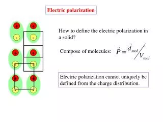
PHENOMENOLOGICAL THEORY OF LEANER DIELECTRIC IN TIME-DEPENDENT FIELDS The dielectric response functions. Superposition principle. A leaner dielectric is a dielectric for which the superposition principle is valid, i.e. the polarization at a time to due to an a electric field with a time-dependence that can be written as a sum E(t)+E’(t), is given by the sum of the polarization’s P(to) and P’(to) due to the fields E(t) and E’(t) separately. Most dielectrics are linear when the field strength is not too high. The superposition principle makes it possible to describe the polarization due to an electric field with arbitrary time dependence, with the help of so-calledresponse functions (t) . (t) is called thestep-response functionor decay functionof the polarization.

For a linear dielectric this response that the total polarization is given by: At t=0 In principle, both a monotonously decreasing and oscillating behavior of (t-t’) are possible. For high values of t, Pwill approximate the equilibrium value of the polarization connected with the static field E. From this it follows that where, called pulse-response function of polarization. This equation gives the general expression for the polarization in the case of a time-dependent Maxwell field.

Let us consider now the time dependence of the dielectric displacement Dfor a time dependent electric field E. For the linear dielectrics the dielectric displacement is a linear function of the electric field strength and the polarization, and for those dielectrics where the superposition principle holds for P, it will also hold for D. Thus, we can write for D analogously to P(t) with The relation between p and D is the following:

And the relation between p and D is: The unit step function in implies that there is an instantaneous decrease of the function D (t-t’), from the value D (0)=1 to a limit value given by: In contrast the step-response function of the polarization cannot show, in principle, such an instantaneous decrease, since any change of the polarization is connected with the motion of any kind of microscopic particles, that cannot be infinitely fast.

The complex dielectric permittivity. Laplace and Fourier Transforms. Let us consider the time dependence of the dielectric displacement Dfor a time dependent Electric field: Applying to the left and right parts the Laplace transform and taking into account the theorem of deconvolution we can obtain: (2.18) where (2.19) (s=+i; 0 and we’ll write instead of sin all Laplace transforms i).

Taking into account the relation (2.20) we can rewrite (2.22) in the following way: (2.20) From another side complex dielectric permittivity can be written in the following form: (2.21) The equation (2.19) justifies the use of the symbol for the dielectric constant of induced polarization, since for infinite frequency the Laplace transform vanishes, and the expression becomes equal to . The real part of complex dielectric permittivity ’() is associated with real part of Laplace transform of orientation pulse-response function: (2.22) and the imaginary part of complex dielectric permittivity ’’() is associated with the negative imaginary part of the Laplace transform of orientation pulse-response function:

(2.23) Let us now reconsider the relationship between time dependent displacement and harmonic electric field: (2.24) We’ll rewrite in this case the relation (2.18) in the following form: (2.25) that can be presented as follows: (2.26) where and

From the equation (2.26) it clearly appears that the dielectric displacement can be considered as a superposition of two harmonic fields with the same frequency, one in phase with electric field and another with a phase difference . The amplitudes of these fields are given by ´E o and ” E o , respectively. Calculation of the energy changes during one cycle of the electric field shows that the field with a phase difference with respect to the electric field gives rise to absorption of energy. The total amount of work exerted on the dielectric during one cycle can be calculated in the following way: (2.27)

Since the fields E and D have the same value at the end of the cycle as at the beginning, the potential energy of the dielectric is also the same. Therefore, the net amount of work exerted by the field on the dielectric corresponds with absorption of energy. Since the dissipated energy is proportional to ”, this quantity is called theloss factor. From (2.27) we find the average energy dissipation per unit of time: (2.28) where called a loss angle. According to the second law of thermodynamics, the amount of energy dissipated per cycle must be always positive or zero. It means that (2.29)

The Kramers-Kronig relations The Kramers-Kronig relations are ultimately a consequence of the principle of causality - the fact that the dielectric response function satisfies the condition: (2.30) It means that there should be no reaction before action. Let us consider again the relations for real and imaginary part of complex dielectric permittivity:

Both ‘() and “() are derived from the same generating function p(t) and that it should be possible in principle to “eliminate” this function and to express ‘() in terms of “(). Let us consider the properties of Hilbert transform: (2.31) In this integral we ignore the imaginary contributions arising from integration through the pole at x=. The first integral is equal to , the second vanishes so that we can obtain: (2.32) This called Hilbert transform

Let us apply this to the ´(): (2.33) In these manipulations we have extended the integration (2.33) to - which is permissible in view of the causality principle. The second integral in (2.33) is equal to “() in view of (2.30) so that one can finally write : (2.34) and similarly: (2.35)

These are the Kramers-Kronig relations which express the value of either “() or ‘() at a particular value of the frequency  in terms of the integral transform of the other throughout the entire frequency range (-, ). In view of what was mentioned above about the even and odd character of these functions, one may change the range of integration to (0, ) and thus obtain the one-sided Kramers-Kroning integrals: (2.36) (2.37)

Relaxation and resonance The decreasing of the polarization in the absence of an electric field, due to the occurrence of a field in the past, is independent of the history of the dielectric, and depends only on the value of the orientation polarization at the instant, with which it is proportional. Denoting the proportionality constant by 1/, since it has the dimension of a reciprocal time, one thus obtains the following differential equation for the orientation polarization in the absence of an electric field: (2.38) with solution: (2.39)

It follows that in this case the step-response function of the orientation polarization is given by an exponential decay: (2.24) where the time constant is called the relaxation time. From (2.24) one obtains for the pulse-response function also an exponential decay, with the same time constant: (2.25) Complex dielectric permittivity as it was shown in last lecture can be written in the following way: Substituting (2.25) into the relation one finds the complex dielectric permittivity: (2.26)

Splitting up the real and imaginary parts of (2.26) one obtains: (2.27) (2.28) These relationships usually called the Debye formulas. Although the one exponential behavior in time domain or the Debye formula in frequency domain give an adequate description of the behavior of the orientation polarization for a large number of condensed systems, for many other systems serious deviations occur. If there are more than one relaxation peak we can assumed different parts of the orientation polarization to decline with different relaxation times k, yielding: (2.29)

(2.30) (2.31) with (2.32) For a continuous distribution of relaxation times: (2.33) (2.34) (2.35) with (2.36)

Equations (2.33) till ( 2.35) appear to be sufficiently general to permit an adequate description of the orientation polarization of almost any condensed system in time-dependent fields. At a very high frequencies, however, the behavior of the response functions at t=0. Any change of the polarization is connected with a motion of massunder theinfluence of forces that depend on the electric field.An instantaneous change of the electric fieldyields an instantaneous change of these forces, corresponding with an instantaneous change of acceleration of the molecular motions  by which the polarization changes, but not with an instantaneous change of the velocities. From this it follows that the derivative of the step-response function of the polarization at t=0 should be zero, which is contrast to the behavior of Eq.(2.3; 2.8 and 2.13) for dielectric relaxation.

Therefore these equations cannot describe adequately the behavior of the response function near t=0, and the corresponding expressions for *() do not hold at very high frequencies (usually 1012 and higher). The behavior of the induced polarization in time dependent fields can be described in phenomenological way. At frequencies corresponding with the characteristic times of the intermolecular motions by which the induced polarization occurs, there are sharp absorption lines, due to the discrete energy levels for these motions. In a first approximation, these absorption lines correspond with delta functions in the frequency dependence of " (2.16)

The corresponding frequency dependence of ‘() is obtained from Kramers-Kronig relations: (2.17) As this expression gives the contribution by the induced polarization, its value for =0 is the dielectric permittivity of induced polarization : (2.18) It follows from (2.17) that for infinitely narrow absorption lines, ‘() becomes infinite at each frequency where an absorption line is situated, the so-called resonance catastrophe. To present these phenomena in terms of polarization it can be assumed that in the absence of an electric field the time-dependent behavior of the polarization is governed by a second-order differential equation: (2.19) which is the same equation as for a harmonic oscillator in the absence of damping, to which the term resonance applies.

s Dielectric properties of water 

For the case of a single relaxation time the points ( , ") lie on a semicircle with center on the axis and intersecting this axis at =s and = . Although the Cole-Cole plot is very useful to investigate if the experimental values of and can be described with a single relaxation time, it is preferable to determine the values of the parameters involved by a different graphical method that was suggested by Cole by plotting of () and ()/ against (). Combining eqns (2.6) and (2.7) one has:

(2.24) (2.25) It follows that both methods yield straight lines, with slopes 1/and , respectively, and ´ intersecting axis at sand .

2.The Cole-Cole equation. The first empirical expressions for *() was given by K.S. Cole and R.H.Cole in 1941: (2.26) (2.27) (2.28)

In time domain the expression for the pulse-response function cannot be obtained directly using the inverse Laplace transform to the Cole-Cole expression. Instead, the pulse-response function can be obtained indirectly by developing (2.26) in series. Taking the Laplace transform to the series one can obtain: (2.29)

3. Cole-Davidson equation In 1950 by Davidson and Cole another expression for *() was given: (2.30) This expression reduces to the Debye equation for =1. Since where=arctgo, separation of the real and imaginary parts is easy, leading to the following expressions for  and : (2.31) (2.32)

From Cole-Davidson equation, the pulse-response function can be obtained directly by taking the inverse Laplace transform: (2.33)

4. The Havriliak-Negami equation (2.34) It is easily seen that this equation is both a generalization of the Cole-Cole equation, to which it reduces for =1, and a generalization of the Cole-Davidson equation to which it reduces for =0. Separation of the real and the imaginary parts gives rather intricate expressions for  and : (2.35) (2.36)

where (2.37)

5. The Fuoss-Kirkwood description Fuoss and Kirkwood observed that for the case of a single relaxation time, the loss factor " () can be written in the following form: (2.38) where m is the maximum value of () in this case given by: (2.39) Eqn.(2.38) can be generalized to the form: (2.40) where  is a parameter with values 0<1 and ”m is now different from . Applying Kramers Kroning relationship, we find that ´min the Fuoss-Kirkwood equation is given by:

(2.41) The parameter  introduced by (2.35) should be distinguished from the parameter in the Cole-Cole equation. An important difference between both parameters is that the Fuoss-Kirkwood equation changes into the expression for a single relaxation time if =1, whereas Cole-Cole equation does so if =0.

6. The Jonscher description The Fuoss-Kirkwood equation can also be written in the form: (2.42) Jonnscher suggested an expression for ”() that is a generalization of Eq. (2.42): (2.43) with 0<m 1, 0 n<1. The Eq. (2.42) makes that the frequency of maximum los is: (2.44)

The quantities 1 and mand 2 and n respectively determine the low frequency and high frequency behavior and can be obtained from a plot of ln”()against ln, which should yield straight lines in the low- and high frequency ranges since one then has respectively: (2.45) (2.46)

New Fitting Software-”DATAMA”

The Problem • Complex systems necessarily entail complex dielectric behaviour. How do we “mine” the nuggets from all the dirt?? • Most Fitting routines consider one variable, frequency, and a parameter set. Yet the energy landscape is governed by temperature. How do we fit over 2 variables and a parameter set?

The Problems of Electric Polarization