CHAPTER 2 - EXPLICIT TRANSIENT DYNAMIC ANALYSYS
160 likes | 414 Views
CHAPTER 2 - EXPLICIT TRANSIENT DYNAMIC ANALYSYS. CONTENTS. Explicit Solution Technique Explicit Timestep Explicit Versus Implicit Technology Applicability of Explicit Techniques. EXPLICIT SOLUTION TECHNIQUE. General Technique

CHAPTER 2 - EXPLICIT TRANSIENT DYNAMIC ANALYSYS
E N D
Presentation Transcript
CONTENTS • Explicit Solution Technique • Explicit Timestep • Explicit Versus Implicit Technology • Applicability of Explicit Techniques
EXPLICIT SOLUTION TECHNIQUE • General Technique • Problem in space solved by FEM methods • Problem in time solved by explicit time integration • - many small time increments • Implementation in MSC.Dytran • Problem in space solved by: • Lagrange-Finite Element Technology • Euler-Finite Volume Technology • Problem in time solved by: • Central difference integration
EXPLICIT vs. IMPLICIT TIMESTEP • EXPLICIT • The timestep size is usually set by the requirements to maintain stability of the central difference integration • The timestep must subdivide the shortest natural period of the elements in the mesh. • Every transient is automatically resolved • IMPLICIT • The solution is unconditionally stable, so the timestep size is dictated by the required accuracy • The timestep must subdivide the shortest natural period of interest in the structure • High transients (e.g. pressure spikes) may not be resolved • IMPLICIT TIMESTEP >> EXPLICIT TIMESTEP • The timestep for an implicit analysis will normally be 10 to 100 times greater than that for an explicit analysis
EXPLICIT TIMESTEP • Timestep must Subdivide Smallest Natural Period of the Mesh • The timestep used by MSC.DYTRAN must be smaller than the smallest natural period of the mesh. Imagine doing an eigenvalue analysis with the same mesh and extracting every possible mode. The timestep must be smaller than the period associated with the highest natural frequency given. The mode shape associated with this eigenvalue is typically one grid point oscillating on the stiffness of the elements to which it is attached. • Courant Criterion • Since it is impossible to do a complete eigenvalue analysis every cycle to calculate the timestep, an approximate method, known as the Courant Criterion, is used. This is based on the minimum time for a stress wave to cross on elements. • It depends on the smallest element dimension, L • where c is the speed of sound through the element material and S is the timestep Scale Factor (<1). • For 1-D elements:
L L D Implicit Integration t D £ t c c F L: smallest element length L D £ t c D t: time step t Force c: sound speed L D ³ t c TIME INTEGRATION Explicit Integration - Small time step - Bigger time step Explicit: Implicit: -No big matrices and - Big matrices and matrix inversion required matrix inversion by having a diagonal - Solution procedure complicated with increasing degree of nonlinearities matrix (lumped mass) -Robust solution procedure even for high degree of nonlinearities
TIMESTEP EXAMPLE Consider a rectangular steel cantilever beam: • EXPLICIT • Minimum element dimension, L = 3.33 mm • Speed of sound, c = 5113 m/s • Timestep = 0.9 L/c = 0.586 microseconds • IMPLICIT • Assume interest up to the third mode • Frequency = 3643 rad/s; period = 1.725 milliseconds • For accuracy, subdivide the period by 20 • Timestep = 86.2 microseconds • IMPLICIT TIMESTEP = 147 x explicit timestep
EXPLICIT VS IMPLICIT TECHNOLOGY • EXPLICIT codes are relatively more efficient for problems with the following characteristics: • Short duration • Computational cost increases linear with problem time, but already small problem times need a lot of time integration steps • Large number or extent of non-linearities • Computational cost remains the same, while for an implicit method the CPU time increases exponentially • Large problem size • Computational cost increases linear with problem size. CPU time increases by a factor of two when number of elements is doubled
COMPUTATIONAL EFFICIENCY IMPLICIT VS EXPLICIT
APPLICABILITY OF EXPLICIT TECHNIQUES • NONLINEAR • Large Displacement • The model can undergo large translations and rotations. There is no small displacement option in MSC.Dytran, but small displacement analysis is not precluded • Contact and Coupling • These interactions allow the simple modeling of complex interactions between two or more separately meshed bodies • Plasticity • A large number of material models are available to model a wide range of material behavior. • Materials as diverse as metals, alloys, plastics and composites can be simulated
APPLICABILITY OF EXPLICIT TECHNIQUES (Cont’d) • Large strain formulation • Most elements have large strain formulation. An option allows the shell elements to get thinner due to membrane straining • Failure • Material flow • In cases where extreme material deformation takes place Euler with strength can be used • TRANSIENT AND DYNAMIC • MSC.Dytran is most suitable for short term events such as explosions and high speed impact • It is intended for dynamic events. Static problems can be analyzed quasi-statically, but the technique is only cost effective if the problem incorporates significant non-linearities