Quantifying knee osteoarthritis
Quantifying knee osteoarthritis. Alice Chuang April 28, 2011 En 250. Introduction. Osteoarthritis increasing in aging population Imaging techniques: Radiography (X-ray) – golden standard, qualitative MRI - quantitative, gaining popularity Spectroscopy Ultrasound


Quantifying knee osteoarthritis
E N D
Presentation Transcript
Quantifying knee osteoarthritis Alice Chuang April 28, 2011 En 250
Introduction • Osteoarthritis increasing in aging population • Imaging techniques: • Radiography (X-ray) – golden standard, qualitative • MRI - quantitative, gaining popularity • Spectroscopy • Ultrasound • Difficult to quantify progress • Joint space width – thickness of articular cartilage • Osteophyte formation – bony protrusion • Kellegren-Lawrence scale for severity of disease
Approach • Fully automatic quantification of knee osteoarthritis severity on plain radiographs. Oka H, Muraki S, et al. Osteoarthritis Cartilage. 2008 Nov;16(11):1300-6. • KOACAD – Knee osteoarthritis computer-aided diagnosis • Thresholds normalized to Kellegren-Lawrence scale based on cohort of 2975 Japanese adults
KOACAD A) Boundaries C) Osteophyte area B) Joint space width, area D) Femorotibial angle
KOACAD Part 1 A) Original image B) Filtered image C) Region of interest Vertical neighborhood difference filter D) Upper rim = femoral condyle Vertical filtering with 3x3 square neighborhood difference filter
KOACAD Part 2 E) Lower rim = Margins of tibial plateau Anterior and posterior margins averaged F) Straight regression line drawn of lower rim G) Joint space area: inside rim, outside rim Inner: Intersection of regression line, lower rim H) Minimum joint space width Minimum vertical space distance
KOACAD Part 3 I) Protrusion Femur, tibia outlined by 3x3 square horizontal neighborhood difference filter J) Osteophyte area = protrusion (inflection point) K) Middle lines from outline of femur, tibia L) Femorotibial angle: axes of femur, tibia Straight-line regression of middle lines
Goal of Project • Create a Matlab program mimicking KOACAD • Quantify disease state of osteoarthritis • Use 2D radiographs • Successes • mJSW – minimum joint space width • JSA – joint space area • FTA – femorotibial angle • Future • Osteophyte area – protrusions near joint • Automation • Filter images
First results: Test images • Simple cartoon images to test Matlab program • Top image, results in pixels • Left • JSA (joint space area) = 24 • min JSW (joint space width) = 1 • Right • JSA = 27 • min JSW = 1 • Bottom, result in degrees • FTA (femorotibial angle) = 178.2
Test images • Top, joint space in pixels • Left • JSA = 462 • min JSW = 6 • Right • JSA = 154 • min JSW = 7 • Bottom, angle in degrees • FTA = 173.7 • Test images show that Matlab program works on idealized images
Process: Boundaries • Vertical difference filter • User control • Threshold as percent of intensity • Upper: femoral condyle • Lower: tibial plateau • Linear regression • Inner: intersection of regression line and tibia • Outer: lateral joint border
Joint Space Characterization • Joint space width (JSW) • Vertical distance in pixels • Minimum JSW • Left: mJSW = 7 • Right: mJSW = 7 • Joint space area (JSA) • Number of pixels • Sum of all JSW • Left: JSA = 682 • Right: JSA = 1076 • Can normalize pixel values
Joint Space Results • Successes • Upper, lower, inner, and outer bounds identified • More shading on lateral sides of joint • Adjusting threshold for vertical neighbor difference • Summing algorithm for Joint Space characterization • Difficulties • Slanted alignment of images • Background noise unfiltered • Dimensions vary • Manual zooming-in is labor intensive
Joint Space Results Left JSA = 240 mJSW = 11 Right JSA = 1377 mJSW = 11 Left JSA = 371 mJSW = 5 Right JSA = 808 mJSW = 5 Left JSA = 23041 mJSW = 62 Right JSA = 4869 mJSW = 60 Left JSA = 10749 mJSW = 13 Right JSA = 6746 mJSW = 26
Test image: FTA • Top, results in pixels • Left • JSA = 462 • min JSW = 6 • Right • JSA = 154 • min JSW = 7 • Bottom, result in degrees • FTA (femorotibial angle) = 173.7
Process: Midline Regression • Horizontal difference filter • User control • Intensity threshold • Medial regression lines • Femur – blue • Tibia – green
Femorotibial Angle • Regression lines • Slope m • m1 – Femur , blue • m2 – Tibia, green • tan(FTA) = (m1 – m2) (1 + m1*m2) • FTA = 169.4 degrees • Same limitations as JSA • Intensity distribution • Highly variable
Femorotibial Angle Results FTA = 172.8 FTA = 176.4
Femorotibial Angle Results FTA = 169.6 FTA = 155.8
Combining analyses • Example of normal knee • Joint space evaluation • Left • JSA (joint space area) = 371 • min JSW (joint space width) = 5 • Right • JSA = 808 • min JSW = 5 • Femorotibial angle • FTA = 171.2 degrees
Combining analyses • Osteoarthritic knee • Right joint space undetectable • Joint space evaluation • Left • JSA (joint space area) = 884 • min JSW (joint space width) = 7 • Right • JSA = 19 • min JSW = 7 • Femorotibial angle • FTA = 169.4 degrees
Conclusion • Numerical comparison of 2D x-rays • Osteoarthritic mJSW and JSA pixel values • FTA – angle of joint bones possible sign of osteoarthritis • Future improvements • Osteophyte area, as done in KOACAD • Image quality • Intensity distribution • Background signals • Automation • Filtering • Threshold detection • Atlas mapping • Compare with 3D imaging
References Primary source: • Oka H, Muraki S, Akune T, Mabuchi A, Suzuki T, Yoshida H, Yamamoto S, Nakamura K, Yoshimura N, Kawaguchi H. Fully automatic quantification of knee osteoarthritis severity on plain radiographs. Osteoarthritis Cartilage. 2008 Nov;16(11):1300-6. Epub 2008 Apr 18. Additional sources: • Oka H, Muraki S, Akune T, Nakamura K, Kawaguchi H, Yoshimura N. Normal and threshold values of radiographic parameters for knee osteoarthritis using a computer-assisted measuring system (KOACAD): the ROAD study. J Orthop Sci. 2010 Nov;15(6):781-9. Epub 2010 Nov 30. • Cooke TD. Re: "Fully automatic quantification of knee osteoarthritis severity on plain radiographs". Authors: H. OKA et al. Osteoarthritis and Cartilage (2008) 16, 1300-1306. Osteoarthritis Cartilage. 2009 Sep;17(9):1252-3; author reply 1254. Epub 2009 Mar 28. • Johansson A, Sundqvist T, Kuiper JH, Öberg PÅ. A spectroscopic approach to imaging and quantification of cartilage lesions in human knee joints. Phys Med Biol. 2011 Mar 21;56(6):1865-78. Epub 2011 Mar 1. • Dodin P, Pelletier JP, Martel-Pelletier J, Abram F. Automatic Human Knee Cartilage Segmentation from 3D Magnetic Resonance Images. IEEE Trans Biomed Eng. 2010 Jul 15. [Epub ahead of print] • Bowers ME, Trinh N, Tung GA, Crisco JJ, Kimia BB, Fleming BC. Quantitative MR imaging using "LiveWire" to measure tibiofemoral articular cartilage thickness. Osteoarthritis Cartilage. 2008 Oct;16(10):1167-73. Epub 2008 Apr 14.
Knee X-ray Sources Primary image source: • Dr. Braden Fleming, Coro Research Center Additional osteoarthritic knee x-rays: • http://www.mayoclinic.com/images/image_popup/mcdc7_kneearthritis.jpg • http://4.bp.blogspot.com/_uC-1Is5ZK44/S-wAlZJ0X9I/AAAAAAAAAQY/w7KHexuDZqA/s1600/Knee%2520X-Ray.jpg • http://3.bp.blogspot.com/_vT13IccOEqM/TL87gkX7JGI/AAAAAAAAASo/8HLvpat1nvo/s1600/89.jpg • http://www.ispub.com/ispub/ijos/volume_5_number_1_27/patella_refashioning_during_tkr_in_patient_with_previous_bilateral_patellectomy_using_bone_cuts/tkr-fig1.jpg • http://www.ispub.com/ispub/ijos/volume_5_number_1_27/patella_refashioning_during_tkr_in_patient_with_previous_bilateral_patellectomy_using_bone_cuts/tkr-fig1.jpg • http://www.hipandkneespecialist.com/knee_arth1B%20Nourbash.gif • http://www.sciencephoto.com/images/showFullWatermarked.html/C0075866-X-Rays_of_Normal_and_Degenerative_Knees-SPL.jpg?id=670075866 • http://www.hwbf.org/hwb/conf/mill1/981030.jpg Additional normal knee x-rays: • http://img.photobucket.com/albums/v110/shanbhag/AchesandJoints/ANJ3-KneeXray-s.jpg • http://fiftyone43four.files.wordpress.com/2010/06/knee_xray_normal.jpg • http://imagecache6.allposters.com/LRG/30/3041/GZPBF00Z.jpg • http://www.sciencephoto.com/images/showFullWatermarked.html/C0075866-X-Rays_of_Normal_and_Degenerative_Knees-SPL.jpg?id=670075866 • http://www.health.com/health/static/hw/media/medical/hw/h9991217.jpg • http://4.bp.blogspot.com/_aG90Nx5mMjw/TSI5OmNwlVI/AAAAAAAAB6s/ZHfANxI-m9A/s640/normal-knee-xray.jpg • http://www.hwbf.org/hwb/conf/mill1/981030.jpg • http://www.stryker.mudbugmedia.com/images/library/stryker_xrays/normal_knee_xray.jpg