Download
1 / 26
320 likes | 911 Views
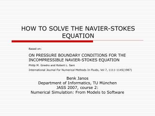
HOW TO SOLVE THE NAVIER-STOKES EQUATION. Based on: ON PRESSURE BOUNDARY CONDITIONS FOR THE INCOMPRESSIBLE NAVIER-STOKES EQUATION Phlilp M. Gresho and Robert L. Sani International Journal For Numerical Methods In Fluids, Vol 7, 1111-1145(1987). Benk Janos Department of Informatics, TU München

E N D
HOW TO SOLVE THE NAVIER-STOKES EQUATION Based on: ON PRESSURE BOUNDARY CONDITIONS FOR THE INCOMPRESSIBLE NAVIER-STOKES EQUATION Phlilp M. Gresho and Robert L. Sani International Journal For Numerical Methods In Fluids, Vol 7, 1111-1145(1987) Benk Janos Department of Informatics, TU München JASS 2007, course 2: Numerical Simulation: From Models to Software
Content • Short introduction • Analysis of the continuum equation • Pressure Poisson equation • Boundary conditions • Discrete approximation to the continuum equation
Short introduction - Important field of application of the numerical simulation - The flow is a result of different physical processes - Numerical flow simulation has a various fields of application, real scenario simulations. http://www.cfd-online.com/Links/misc.html#picts
Analysis of the continuum equation The momentum equation for incompressible fluids (1) The second equation is the continuity equation (2) If it would be compressible fluid (3)
Analysis of the continuum equation Each part from the (1) equation has a contribution to the momentum The velocity change describing the acceleration of a infinite mass point. It must be in balance with … … the convective term describing the frictionless acceleration induced by the velocity filed. … the gradient of the pressure. (by definition is an acceleration)
Analysis of the continuum equation This component reflects the interior drag of the fluid. Re is the Reynolds number. The drag appears between two layers of fluid with different velocity. - The friction force is acting against the velocity gradient - This laminar flow, which opposes turbulent flow
Analysis of the continuum equation • At gas flow this term can be neglected, but by fluids not (e.g. honey) • The internal friction is also called viscosity, which characterize each fluid. vs - mean fluid velocity, L - characteristic length, μ - (absolute) dynamic fluid viscosity, ν - cinematic fluid viscosity: ν = μ / ρ, ρ - fluid density. source:http://en.wikipedia.org/wiki/Reynolds_number
Analysis of the continuum equation External accelerations. ex: gravity This component contains other forces which are not represented by other terms We need boundary conditions so that the problem will be solvable - Ω is the fluid domain , and is bounded by Γ
Analysis of the continuum equation w is the velocity on the boundary (Dirichlet BC) u = w(x,t) on Γ - This leads to the BC for the continuity equation (mass conservation) n is the normal vector on the boundary (4) We consider the initial situation t=0
Analysis of the continuum equation Accordingly to equation (2), this holds also for the initial velocity field in Ω In 2D we have the following vectors on the boundary n -> normal vector τ -> tangential component
Pressure Poisson equation • Calculate the pressure field from a velocity field. • Want to have a relation between pressure and velocity, in discrete and in continuum time. • Show one way to get the Poisson equation
Pressure Poisson equation We start with equation (1), and we neglect external influences First we apply the divergence operator, so we get: We use the following expression to process further the equation:
Pressure Poisson equation And because: for any (differentiable) vector field. We obtain: We obtain the pressure Poisson equation:
Pressure Poisson equation A slightly modified system has to be solved for the discrete time dependent solution. Discretizing the first(1) equation: Expressing u+ and insert the solution in the second(2) equation, we can calculate the pressure
Boundary condition • To complete the specification of the problem for the pressure, we must set BC’s (boundary conditions) on Γ • It is important how we include the boundary conditions in our system. • For the boundary condition we need a scalar value, so we have 2 choice: either the normal or the tangential projection
Boundary condition First we choose the normal component: (Neumann) on Γ The BC with the tangential component (Dirichlet): on Γ It has been proven that these 2 conditions are equivalent. We can calculate the pressure up to an arbitrary additive constant!!!
Boundary condition The question is: When the original NS problem is well-posed, so is the associated Poisson/Neumann problem? Here is the proof: We start with the first equation and in Ω also on Γ
Boundary condition Apply Green formula, and we obtain an integration on the boundary Substituting the left side, we obtain the following equation
Boundary condition Finally we obtain the following equation w is representing the velocity on the boundary. We obtained the mass conservation law (4), which is satisfied. This means that our transformed problem is also well posed.
Discrete approximation to the continuum equation • Build the system of equations • We want to calculate the real pressure, on the boundary • Check whether the system has a correct boundary result
Discrete approximation to the continuum equation We can write the momentum and the continuity equation in the following discretized general way: M – mass matrix, (for equidistant discretization is the unit matrix) A – advection matrix G – gradient matrix K – diffusion matrix D – divergence matrix
Discrete approximation to the continuum equation f(t) , g(t) - represents the effects of the boundary Dirichlet conditions on velocity. We use the following notations and equalities: Denoting G with C we get:
Discrete approximation to the continuum equation We consider the hydrostatic pressure P=(1->1), the system has a solution if g(t) satisfies the following condition. From the above define system we can derive the discrete pressure Poisson equation:
Discrete approximation to the continuum equation We use the following staggered mesh: We apply the continuity equation for cell with P0(on the boundary)
Discrete approximation to the continuum equation Expressing all 3 terms (ue is known on the boundary) from the momentum equation. We use Taylor expansion to express the velocity at the “fictive” nodes, and we use the boundary velocities With l, h ->0 (on the limit) we get the real boundary condition.