Download

1 / 22
220 likes | 386 Views
Reliability Prediction of Electronic Boards by Analyzing Field Return Data. Authors : Vehbi Cömert (Presenter) Mustafa Altun Hadi Yadavari Ertunç Ertürk. P erforming a reliability analysis using a real field return data

E N D
ReliabilityPrediction of Electronic BoardsbyAnalyzing Field Return Data Authors: Vehbi Cömert (Presenter) Mustafa Altun Hadi Yadavari Ertunç Ertürk
Performing a reliability analysis using a real field return data • Motivation: Modeling hazard rate curveandmakingaccuratereliabilityprediction
Introduction • Field Return Data • Electronics Reliability • Filtering • Field return data may have obvious and hidden errors. • Surveying accuracy of the field return data to find errors • Based on beta parameter of Weibull distirubtion • Modeling of hazard rate curve • Reliability prediction with filtered field return data • Investigation of distributions that fits to data. • Change of hazard rate shape with respect to ‘Time to Failure’ • Two phase hazard rate curve
Field Return Data • The field return data ,that we use, belongstoArçelik (Beko), one of thebiggestwhiteapliancecompany in Europe • It is a warranty data andincludes - 1 million sales - 3000 warranty claims - Wehavefirst 54 monthsof the data • Warranty involves 36 months.
ElectronicsReliability • Good reliability • Expected long life • Usually catastrophic failures • Decreasingorconstant hazard rate • Hard to see wear out signs
Filtering Eliminating errors in field return data Step 1 : Eliminating Obvious Errors Step 2 : Eliminating Hidden Errors Stage 1: Forward analysis Stage 2: Backward analysis Stage 3: 6-month analysis
Errors in field return data • Obvious error : The errors that can be seen easily by checking claims • Hidden error : The errors that cannot be seen at first glance What can be a hidden error? Missing Claims
Filtering Process • To ensure the accuracy of the analysis, errors must be eliminated !!! Step 1 : Obvious errors must be filtered by checking hand Records with; Unknown assembly date Unknown return date Zero time to failure Negative time to failure Unreasonable time to failure
FilteringProcess • Step -2: Investigatethe data using Weibull distribution to find hidden errors. • Weibull distribution parameters; - Beta(): shape parameter - Alfa (): scale parameter <1 Decreasing Failure Rate =1 Constant Failure Rate >1 Increasing Failure Rate
Filtering Process Assembly date/Month • Step -2 stage1 : Forward Analysis 1 6 12 18 24 30 36 42 48 54 valuesforforward time intervals Weibull Fitting problematic
FilteringProcess Assembly date/Month • Step-2 stage-2: Backwardanalysis 1 6 12 18 24 30 36 42 48 54 valuesforbackward time intervals Lack of return data towardend of the time
FilteringProcess Assembly date/Month • Step-2 stage-3: 6 - monthperiodsanalysis 0 6 12 18 24 30 36 42 48 54 valuesfor 6-month periods problematic
FilteringProcess valuesforbackward time intervals valuesforforward time intervals problematic valuesfor 6-month periods First threeintervals (1-18 months) should be filtered. problematic
Modeling of hazard rate curve To obtain an accuratehazard rate curve Searchingpointswherethehazard rate tendencychanges Forward and Backward analysis
Modeling of Hazard Rate Curve Change Point (): Fromdecreasing rate trend toconstant rate trend
Modeling of Hazard Rate Curve • Method to find change point via Reliasoft Weibull++ • Analyzing filtered field return data in terms of time to failure (TTF) - Using ‘’best fit’’ option in Weibull++andfitting with respect to different time intervals. - Tryingtofind the point where the best fitting distribution changesbyshowingdifferent hazard rate trend
Modeling of Hazard Rate Curve Time to Failure/month • Forward analysis 1 2 3 4 5 6 7 8 …………………………… Mf……………………………………………..…………………………..36 includesfieldreturnsthat can haveall TTF valuesbetween 1 andMf Mostlikelihooddistribution • Results : At end of each interval analysis, decreasing hazard rate trend was observed for this filtered data. Weibull++ offered most commonly Weibull distribution in addition to Lognormal and Gamma distributions What is the hazard rate trend?
Modeling of Hazard Rate Curve • Backward analysis Results : - Exponential distribution for , constant hazar rate - Weibull, Lognormal and Gamma Distribution for decreasinghazard rate 1 2 3 4 5 6 7 8 …………………………… Mb …………………………………….……………33 34 35 36 includesfieldreturnsthat can haveall TTF valuesbetweenMband 36 month
Modeling of Hazard Rate Curve M > 14 Exponential Distribution M < 14 Weibull Distribuiton
Modeling of Hazard Rate Curve • : overall hazar rate function : indicatorfunction
Conclusion • FILTERING • A systematic approach is offered for elimination errors in field return data • To determine hidden errors. • 1) Forward Analysis • 2) Backward Analysis • 3) 6-month Analysis • 18 months at begining of the data seem as problematic • MODELINGOF HAZARD RATE CURVE • Welookforchange of hazard rate tendency • 1) Forward Analysis • 2) Backward Analysis • In the forward analysis we didn’t see a change in the hazard rate shape • But in the backward analysis,exponential distribution fits best between14and 36 months • Thisstudywill be usedby Arçelik • Usefullforhighvolumesales • Thismethods can be generalizedforallfieldreturndatas