Information Cascade
Information Cascade. Priyanka Garg. OUTLINE. Information Propagation Virus Propagation Model How to model infection? Inferring Latent Social Networks Inferring edge influence Inferring influence volume. Information Propagation. How information/infection/influence flows in the network?


Information Cascade
E N D
Presentation Transcript
Information Cascade Priyanka Garg
OUTLINE • Information Propagation • Virus Propagation Model • How to model infection? • Inferring Latent Social Networks • Inferring edge influence • Inferring influence volume
Information Propagation • How information/infection/influence flows in the network? • Epidemiology: • Question: Will a virus take over the network? • Type of virus: • Susceptible Infected Susceptible (SIS) • Example: Flu • Susceptible Infected Removed (SIR) • Example: Chicken-pox , deadly disease • Viral Marketing: • Once a node is infected, it remains infected. • Question: How to select a subset of persons such that maximum number of persons can be influenced?
How to model infection? • Simple model: • Each infected node infects its neighbor with a fixed probability. • SIS: • A node infects its neighbor with probability b (how infectious is the virus?) • Node recovers with probability a (how easy is it to get cured?) • Strength of virus = b/a • Result: If virus strength < t then virus will instinct eventually. t = 1/largest eigen value of adjacency matrix A.
How to model infection? • Independent Contagion Model • Each infected node infects its neighboring node with probability pij. • Threshold Model • Each infected node i infect its neighboring node j with weight wij. • The node j becomes active if ∑j=neigh(i)wij > thi. • thi is the threshold of node i.
How to model infection?: General Contagion Model • General language to describe information diffusion. • Model: • S infected nodes tried but failed to infect node v. • New node u becomes infected. • Probability of node u successfully influencing node v also depends on S. pv(u, S) • Example • Node becomes active if k of its neighbors are active. ie. if |S + 1| > k then pv(u, S) = 1 else 0 • Independent Cascade: pv(u,S) = p(u,v) • Threshold model: if (p(S,v) + p(u,v)) > t then pv(u,S) = 1 else 0
How to model infection?: General Contagion Model • Can also model the diminishing returns property • S>T then Gain(S + u) < Gain (T + u) • Gain = Probability of infecting neighbor j
Challenges in using these models • Problem under consideration • Viral marketing: How to select a subset of persons such that maximum number of persons can be influenced? • How to find the infection probability/weights of every edge?
Inferring infection probabilities • We know the time of infections over a lots of cascades. • Train: • Maximize the likelihood of node infections over all the nodes in all the cascades. • Likelihood = ∏c∏iPi,c • Pi = P(i gets infected at time ti| infected nodes) • Independent Contagion Model • Pi=At least one of the already infected node infects node i • Pi= 1 - ∏j(1-(probability of infection from node j to node i at time ti))
Inferring infection probabilities • Variability with time: • Infection probabilities vary with time. Let w(t) is the distribution which captures the variability with time. • Probability of node j infecting node i at time t is w(t-tj)*Aji. Here tj is the infection time of node j. • Thus: • Pi= 1 - ∏j(1- w(ti-tj)Aji) • The log-likelihood maximization problem can be shown to be a convex optimization problem
Another approach: more direct • Find number of infected nodes at any time t? • Number of infected nodes at time t depends only on number of already infected nodes. • Model: • V(t) is the number of nodes infected at time t • V(t+1) = ∑u=1,N ∑l=0,L-1 Mu(t-l) Iu(l+1) • Mu(t) = 1 if node u is infected at time t • Iu(t) = Infection variability with time • Minimize the difference between V(t) and observed volume at every time t. • Accounting for novelty: • V(t+1) = α(t)∑u=1,N ∑l=0,L-1 Mu(t-l) Iu(l+1)
SIS • Let • pit = P(i is infected at time t) • tit = P(i doesn’t receive infection from its neighbor) • tit = ∏j=neigh(i) (pj(t-1) (1-b) + 1 – pj(t-1)) • 1-pit=P(i is healthy at t-1 and didn’t receive infection) + P(i is infected at t-1 and got recovered and didn’t receive infection) + P(i is not infected at t-1 but got cured after infection at t). • 1 – pit = (1-pi(t-1)) tit + pi(t-1)a tit + (1-pi(t-1))tita 0.5