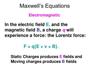
Maxwell’s Equations
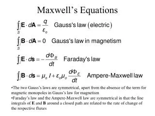
Maxwell’s Equations. The complete equations in differential form: with the constitutive relations: Other important forms that we will see: (1) Integral form (using Stokes and Gauss’s theorems) (2) Phasor/Frequency domain form. Maxwell’s Equations. Time-independent (Static) Forms:


Maxwell’s Equations
E N D
Presentation Transcript
Maxwell’s Equations • The complete equations in differential form: • with the constitutive relations: • Other important forms that we will see: • (1) Integral form (using Stokes and Gauss’s theorems) • (2) Phasor/Frequency domain form
Maxwell’s Equations Time-independent (Static) Forms: The electric and magnetic fields decouple; they can be treated independently! This observation is the starting point for electrostatics and magnetostatics When can we neglect the time variations? In the same limit that circuit theory holds
Maxwell’s Equations • Time-independent (Static) Forms: • The electric and magnetic fields decouple; they can be treated independently! • This observation is the starting point for electrostatics and magnetostatics • So, why bother with statics? • (1) Important applications: near fields of radiating systems; inductors and capacitors; electrostatic discharge • (2) Visualizing fields: The full system is complex; it contains radiative contributions; charge contributions; current contributions. It is important to learn about each of them separately.
Constitutive Relations • Where do they come from? • There are two kinds of charge:free (these flow in conductors) [This charge is included in rV] • bound (these are dipole charges in dielectrics)[This charge is what determines e!] • In statics, the bound charges alwaystend to cancel the free charges. • Thus, we have: • NOTE: D = field response to free charge E = field response to total charge Ulaby Figure 1-6
Constitutive Relations • Where do they come from? • There are two kinds of charge:free (these flow in conductors) [This charge is included in rV] • bound (these are dipole charges in dielectrics)[This charge is what determines e!] • Approximate calculations of e are possible semi-classically • BUT • Exact calculations usually require quantum mechanics An important exception is plasmas,which can be treated classically Ulaby Figure 1-6
Constitutive Relations boundcurrent J freecurrent • Where do they come from? • There are also two kinds of current:free (these flow in conductors) [This current is included in J ] • bound (in magnetic materials)Important note: Static current always flows in loops! • That is a consequence of ·B = 0 • NOTE: H = field response to free current B = field response to total current
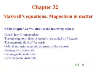
Constitutive Relations boundcurrent J freecurrent • Where do they come from? • There are also two kinds of current:free (these flow in conductors) [This current is included in J ] • bound (in magnetic materials)BUT: the behavior of magnetic materials is complicated even in the static limit! • There are three kinds of magnetic materials • Ferromagnetic (permanent magnets) • Paramagnetic • Diamagnetic
Constitutive Relations Ulaby boundcurrent J freecurrent • Ferromagnetism: B mH • These materials are highly nonlinearand have hysteresis • Quantum mechanics must be used to explain this phenomenon; no semi-classical explanation is possible • Paramagnetism: B mH • A small amount of hysteresis may be present • The bound flow is in the same direction asthe free flow and enhances it (m > m0 ) • Semi-classical explanation is not possible
Constitutive Relations boundcurrent J freecurrent • Diamagnetism: B= mH • No hysteresis is present • The bound flow is in the opposite direction from the free flow anddecreases it (mr< 1) • Semi-classical explanation is possible • Fortunately, in almost all dielectric materials: B = m0H
Charge and Current Distributions Volume charge density Conversely, we have in a finite volume v: It is useful to define analogous surface and line charge densities Surface and line charge densities The converses are:
Charge and Current Distributions Surface Charge Distribution: Ulaby Example 4-2 Question: A circular disk of electric charge is azimuthally symmetric and increases linearly with r from 0 to 6 C/m2 at r = 3 cm. What is the total charge on the surface? Answer: We have so that Ulaby Figure 4-1(b)
Charge and Current Distributions Current density The increment of current that flows through a surface Ds in a time Dt is given by: The converse is: Ulaby Figure 4-2
Charge and Current Distributions • Coulomb’s Law: • An isolated charge q induces an electric field E at every point in space and at the point P, the field E is given by Ulaby Figure 4-2
Charge and Current Distributions • Coulomb’s Law: • An electric field E at a point P in space, which may be due to one charge or many charges, induces a force on a charge q that is given byNOTE: The only way to detect the presence of a field (electric or magnetic) is by the force that it exerts on charges.— In this sense, the fields are an abstraction, albeit a very useful one
Charge and Current Distributions • Multiple Point Charges: • When we have multiple point charges, we add the field contributions from each of them vectorially • IMPORTANT NOTE: A charge does notcontribute to the electric field at its own location! Ulaby Figure 4-4
Charge and Current Distributions Electric Field Due to Two Point Charges: Ulaby Example 4-3 Question: Two point charges with q1 = 2 × 10⁻⁵ C and q2 = –4 × 10⁻⁵ C are located at (1, 3, –1) and (–3, 1, –2), respectively, in a Cartesian coordinate system. Find (a) the electric field E at (3, 1, –2) and (b) the force on a charge q3 = 8 × 10⁻⁵ C located at that point. Answer: (a) Since e = e0 and there are two charges, we have with
Charge and Current Distributions Electric Field Due to Two Point Charges: Ulaby Example 4-3 Answer: (a) [continued] After substitution, we find (b) Using the force equation, we have Ulaby 2001
Charge and Current Distributions • Continuous Charge Distributions: • When we have a continuous charge density, each increment of chargecontributes • Integrating over a complete volume, we obtain: • For surface and line distributions, these become Ulaby Figure 4-5
Charge and Current Distributions Example: An Infinite Charge Sheet Question: An infinite plane of charge is located on the x-y plane. What is the electric field at the point P(0, 0, h)? Answer: We will build up the answer in two parts. The first part is to integrate over a ring ofcharge (Ulaby, Example 4-4) and then integrate over many rings. Integration over the ring: Ulaby Figure 4-6
Charge and Current Distributions Example: An Infinite Charge Sheet Answer (continued): Integration over the ring: Due to the symmetry, only the z-component appears! Ulaby Figure 4-6
Charge and Current Distributions Example: An Infinite Charge Sheet Answer (continued): Integration over a circle: Making the replacements, and integrating from r = 0 to r = a, we find Integration over the plane: When a ,we find Ulaby 2001 When h < 0, the answer is the samewith the opposite sign NOTE: This simple, yet important result can also be obtained directly from Gauss’s law Ulaby Figure 4-7