Download
1 / 65
700 likes | 1.01k Views
Variation and weighted residual formulation. Chapter 2. General concepts. Governing equation inΩ Boundary condition Approximate solution :

E N D
General concepts • Governing equation inΩ • Boundary condition • Approximate solution : • Ni(x) is the basis or trial function that must satisfy the BCs • R is amount of error or residual • The better approximation, the lower error or residual • Better accuracy could be obtain by higher order approximation • Better accuracy could be obtain by using more basis functions
Problem Definition heat source Q Distance along rod, x X=0 X=1 T=0 T=0 X Insulation around periphery of bar
The variational method We try to find a function T(x) that minimizes or maximized integrals of The variational formulation of the problem in example (4-1) become
The variational method • The idea is to find the function T(x) that extremizes I • The function T(x) satisfies the original differential equation and boundary conditions • the variational form may be used to obtain solutions to problems that are not readily admitted by the differential formulation • The variational formulation of a physical problem is often referred to as the the weak formulation
Example : • Solving problem posed in the given example by the variational method • Solution • If a mimimum has been found • If a maximum has been found
Variational method 50 40 30 20 10 Comparison of approximate solution to problem posed in the given example Tempreture. T Ritz method ------- Variational method 0 0.2 0.4 0.6 0.8 1.0 Distance along rod, x
Variational calculus • The weighted- residual methods are far easier to apply and can be used even when no variational formulation exists • All variational formulation have a corresponding differential formulation, but, unfortunately , the converse is not true: some differential formulation have no classical variational principle
Variational calculus y B y(x) • The curve that results in the shortest length connecting A and B is shown along with the variation and curve y(x) A x
Variational calculus • The shortest curve that connects two given points • First, we must set an integral I that represents the length of the curve. • An element are length ds from the phythagorean theorem is given by
Variational calculus • a family of curves that connects points A and B in the plane of the figure. • By minimizing the integral I, we will obtian the equation of the line that results in the shortest possible length. y B ds dy A dx total length of the curve from x=a at point A to x=b at point B x=a x=b x
Variational calculus • Function F must satisfy the following differential equation:
Variational calculus • By using the boundary conditions:
Integration by parts • Taylor’s series
The differential of a function • Variation of a function F(x,y,yx) , δx=0
The commutative properties • The commutative property of differentiation and variation operators • Another commutative property is
Miscellaneous Rules of variational calculus • Y and z be any continuous and differentiable functions.
THE EULER-LAGRANGE EQUATIONGEOMETRIC AND NATURAL BOUDARY CONDITIONS • The necessary condition for the existence of an extremum of the functional • Is that its first variation must be zero, or
THE EULER-LAGRANGE EQUATION:GEOMETRIC AND NATURAL BOUDARY CONDITIONS • Rewrite • Therefore becomes
THE EULER-LAGRANGE EQUATION:GEOMETRIC AND NATURAL BOUDARY CONDITIONS • Fixed boundary conditions • Natural boundary conditions EULER-LAGRANGE EQUATION
Example : Variational formulation for the given differential equation • For the problem posed in example 4-1, show that the functional to be extremized • solution
Example : • The value of T is to be held fixed at either end of the interval ,the variation of T or must be zero at these two point • Condition T(0)=0 and T(1)=0, since at these points. This type of boundary condition is referred to as a geometric boundary condition • When on the boundary, we have a natural boundary condition.
Example : Variational formulation for the given differential equation (1)
Example : Variational formulation for the given differential equation (2) • By starting with • For the problem stated in example 4-1 drive I
solution • This may be broken into two separate integrals to give:
solution • We have T=0 at x=0 x=1 • Could be satisfied is when dT/dxis zero on the boundaries, i.e., at x=0 and x=1 in this problem. • dT/dx is zero when insulation is present. • The condition that ∂F/∂Tx is also referred to as a natural boundary condition
Euler-Lagrange equation • The Euler-Lagrange equation was introduced for the class of problems whose functional F providing we also satisfy
One set of natural boundary conditions must be given by While from We must have As another boundary condition geometric boundary condition are given by
Variational formulation Variational formulations exist for only those problems whose differential formulations do not contain odd-ordered derivatives
Weighted Residuals • The method of weighted residuals provides an analyst with a very powerful approximate solution procedure that is applicable to a wide variety of problems, it is the existence of the various weighted residual methods that makes it unnecessary to search for variational formulations to nonstructural problems in order to apply the finite element method to these problems.
General concepts of weighted residuals • Governing equation • Boundary conditions
General concepts of weighted residuals Unknown (but constant) parameters Trial function N arbitrary weighting functions
General concepts of weighted residuals Point collocation Sub domain collocation Most popular weighted-residual methods Least squares Galerkin
Problem Definition heat source Q Distance along rod, x X=0 X=1 T=0 T=0 X Insulation around periphery of bar
The ritz method • R is the residual or error • Trial (basis) function Satisfy the boundary condition Does not grossly violate the physics of problem
The ritz method the first – order approximation T:
Point Collocation • weighting function wi(x) (x-xi) • Defined
Example : • Using the trial function assumed in example 4-1, determine an approximate solution to the problem posed in that example by the point collocation method • Solution Only one trail function is used Only one parameter(namely, a1) Choose the collocation point x1to be in the middle of the domain, or x1=1/2
Example : • Must evaluate this residual at the collocation point or at x1=1/2 and set the result to zero, or • Solving for a1 • Number of unknown parameters must be equal to the number of collocation points
Subdomain Collocation • the weighting functions are chosen to be unity over a portion of the domain and zero elsewhere. Mathematically, the wi(x) are given by
Subdomain Collocation • N integral equations • The different integration domains should be noted • Number of unknowns must be equal to number of integrals or number of subdomains
Subdomain Collocation • Collocation weighted-residual method for three subdomains 1 w3 (x) 0 Ω1 x 1 w2 (x) 0 Ω2 x 1 w1 (x) 0 x Ω3 Ω
Example : • Repeat example 4-1 by using the subdomain collocation method with the same trial function • Since only one parameter is unknown so only one domain must be used which is Ω=[0 1]
Least Squares • The method of least squares requires that the integral I of the square of the residual R be minimized. the integral I is given by
Example : • Resolve (approximately) the problem in example 4-1 by using the least-squares method and the same trail function • There is only one unknown parameter a1