Microsoft Excel 2010
Microsoft Excel 2010. Chapter 8 Working with Trendlines , PivotTable Reports, PivotChart Reports, and Slicers. Objectives. Analyze worksheet data using a trendline Create a PivotTable report Format a PivotTable report Apply filters to a PivotTable report Create a PivotChart report

Microsoft Excel 2010
E N D
Presentation Transcript
MicrosoftExcel 2010 Chapter 8 Working with Trendlines, PivotTable Reports, PivotChart Reports, and Slicers
Objectives • Analyze worksheet data using a trendline • Create a PivotTable report • Format a PivotTable report • Apply filters to a PivotTable report • Create a PivotChart report • Format a PivotChart report Working with Trendlines, PivotTable Reports, PivotChart Reports, and Slicers
Objectives • Apply filters to a PivotChart report • Analyze worksheet data using PivotTable and PivotChart reports • Create slicers to filter PivotTable and PivotChart reports • Format slicers • Analyze PivotTable and PivotChart reports using slicers Working with Trendlines, PivotTable Reports, PivotChart Reports, and Slicers
Project – Eckart Pet Supplies Sales Analysis Working with Trendlines, PivotTable Reports, PivotChart Reports, and Slicers
General Project Guidelines • Identify the trend or trends to analyze with a trendline • Determine the type of trendline to add • Identify the types of questions to ask of your data • Visualize your workbook in various PivotTable and PivotChart layouts • Consider using slicers to filter a PivotTable Working with Trendlines, PivotTable Reports, PivotChart Reports, and Slicers
Creating a 2-D Line Chart • Select the range of cells to be charted • Click the Line button (Insert tab | Charts group) to display the Line gallery • Click the Line with Markers chart type in the 2-D Line area of the Line gallery to insert a 2-D line chart with data markers • Click the Move Chart button (Chart Tools Design tab | Location group) to display the Move Chart dialog box • Click the New sheetoption button (Move Chart dialog box) to select it Working with Trendlines, PivotTable Reports, PivotChart Reports, and Slicers
Creating a 2-D Line Chart • If necessary, double-click the default text in the New sheet text box to select the text • Type the desired chart name • Click the OK button to move the chart to a new sheet • Click the default title to select it • Type the desired chart title and then press the ENTER key • Click the outside of the chart area to deselect the chart Working with Trendlines, PivotTable Reports, PivotChart Reports, and Slicers
Creating a 2-D Line Chart Working with Trendlines, PivotTable Reports, PivotChart Reports, and Slicers
Adding a Trendline to a Chart • Click the chart to select it • Click the Trendline button (Chart Tools Layout tab | Analysis group) to display the Trendlinemenu • Click the More Trendline Options command to display the Format Trendline dialog box • If necessary, click the Trendline Options category in the left pane • Click the desired trendline type • Click the desired options in the Format Trendline dialog box • Click the Close button to add the trendline with the selected options Working with Trendlines, PivotTable Reports, PivotChart Reports, and Slicers
Adding a Trendline to a Chart Working with Trendlines, PivotTable Reports, PivotChart Reports, and Slicers
Creating a Blank PivotTable Report • Click the desired cell containing the data for the PivotTable • Click the PivotTable button arrow (Insert tab | Tables group) to display the PivotTable menu • Click PivotTable to display the Create PivotTable dialog box • Click the OK button to create a blank PivotTable report Working with Trendlines, PivotTable Reports, PivotChart Reports, and Slicers
Creating a Blank PivotTable Report Working with Trendlines, PivotTable Reports, PivotChart Reports, and Slicers
Adding Data to the PivotTable Working with Trendlines, PivotTable Reports, PivotChart Reports, and Slicers
Changing the Layout of a PivotTable Report • Click the Report Layout button (PivotTable Tools Design tab | Layout group) to display the Report Layout menu • Click the desired layout Working with Trendlines, PivotTable Reports, PivotChart Reports, and Slicers
Changing the Layout of a PivotTable Report Working with Trendlines, PivotTable Reports, PivotChart Reports, and Slicers
Changing the View of a PivotTable Report Working with Trendlines, PivotTable Reports, PivotChart Reports, and Slicers
Filtering a PivotTable Report Using a Report Filter • Drag the desired field from the ‘Choose fields to add to report’ area to the Report Filter area in the PivotTable Field List pane • Click the field’s AutoFilter button to display the AutoFilter menu • Click to select the desired criterion • Click the OK button to update the display Working with Trendlines, PivotTable Reports, PivotChart Reports, and Slicers
Filtering a PivotTable Report Using a Report Filter Working with Trendlines, PivotTable Reports, PivotChart Reports, and Slicers
Filtering a PivotTable Report Using Multiple Selection Criteria • Click the AutoFilter button to display the AutoFilter menu • Click the Select Multiple Items check box to prepare for adding a criterion • Click the desired check boxes to select the criterion • Click the OK button to update the display Working with Trendlines, PivotTable Reports, PivotChart Reports, and Slicers
Filtering a PivotTable Report Using Multiple Selection Criteria Working with Trendlines, PivotTable Reports, PivotChart Reports, and Slicers
Removing a Filter from a PivotTable Report • Click and drag the desired button from the Report Filter area in the PivotTable Field List pane to outside of the PivotTable Field List pane to remove the report filter from the PivotTable report Working with Trendlines, PivotTable Reports, PivotChart Reports, and Slicers
Filtering a PivotTable Report Using the Row Label Filter • Click the desired AutoFilter button to display the AutoFilter menu and select the desired field • Click the OK button to update the display Working with Trendlines, PivotTable Reports, PivotChart Reports, and Slicers
Removing a Row Label Filter from a PivotTable Report • Click the AutoFilter button to display the AutoFilter menu • Click the Clear Filter From command to remove the row label filter Working with Trendlines, PivotTable Reports, PivotChart Reports, and Slicers
Formatting a PivotTable Report • Select a cell in the PivotTable • Click the More button in the PivotTable Styles gallery (PivotTable Tools Design tab | PivotTable Styles group) to expand the gallery • Click the desired style • Format the cells as desired using the Format Cells dialog box Working with Trendlines, PivotTable Reports, PivotChart Reports, and Slicers
Formatting a PivotTable Report Working with Trendlines, PivotTable Reports, PivotChart Reports, and Slicers
Switching Summary Functions in a PivotTable • Right-click the desired cell to display the shortcut menu and prepare for changing the summary function • Point to Summarize Values By on the shortcut menu to display the Summarize Values By menu • Click the desired command Working with Trendlines, PivotTable Reports, PivotChart Reports, and Slicers
Switching Summary Functions in a PivotTable Working with Trendlines, PivotTable Reports, PivotChart Reports, and Slicers
Summary Functions for PivotChart Report and PivotTable Report Data Analysis Working with Trendlines, PivotTable Reports, PivotChart Reports, and Slicers
Filtering a PivotTable Report Using Multiple Criteria • Click the AutoFilter button to display the AutoFilter menu • Click the (Select All) check box on the AutoFilter menu to deselect all locations • Click the desired check box to filter • Point to the Value Filters command to display the Value Filters menu • Click the desired command • Enter the desired criteria in the Value Filter dialog box • Click the OK button to apply the filter to the PivotTable report Working with Trendlines, PivotTable Reports, PivotChart Reports, and Slicers
Filtering a PivotTable Report Using Multiple Criteria Working with Trendlines, PivotTable Reports, PivotChart Reports, and Slicers
Removing Multiple Filter Criteria from a PivotTable Report • Click the AutoFilter button to display the AutoFilter menu • Click the Clear Filter From command on the AutoFilter menu to remove the filter criteria Working with Trendlines, PivotTable Reports, PivotChart Reports, and Slicers
Updating the Contents of a PivotTable Report • Click the Refresh button (PivotTable Tools Options tab | Data group) to update the PivotTable Report to reflect the change to the underlying data Working with Trendlines, PivotTable Reports, PivotChart Reports, and Slicers
Customizing the Display of the Field List and Field Headers in the PivotTable Report • Click the Field List button (PivotTable Tools Options tab | Show group) to hide the PivotTable Field List pane • Click the Field Headersbutton (PivotTable Tools Options tab | Show group) to hide the field headers • Click the Options button (PivotTable Tools Options tab | PivotTable group) to display the PivotTable Options dialog box • Click the ‘Autofitcolumn widths on update’ check box to remove the check mark • Click the OK button to turn off the autofitting of column widths Working with Trendlines, PivotTable Reports, PivotChart Reports, and Slicers
Customizing the Display of the Field List and Field Headers in the PivotTable Report Working with Trendlines, PivotTable Reports, PivotChart Reports, and Slicers
Customizing the Display of the +/– Buttons in the PivotTable Report • Right-click a cell containing the +/– button to display the shortcut menu, and then point to Expand/Collapse to display the Expand/ Collapse menu • Click Collapse to collapse the data • Click the +/– Buttons button (PivotTable Tools Options tab | Show group) to hide the expand and collapse buttons in the PivotTable Working with Trendlines, PivotTable Reports, PivotChart Reports, and Slicers
Customizing the Display of the +/– Buttons in the PivotTable Report Working with Trendlines, PivotTable Reports, PivotChart Reports, and Slicers
Creating a PivotChart Report from an Existing PivotTable Report • Select a cell in the PivotTable report • Click the Field List button (PivotTable Tools Options tab | Show group) to display the PivotTable Field List pane • Click the PivotChart button (PivotTable Tools Options tab | Tools group) to display the Insert Chart dialog box • Click the desired chart type • Click the OK button to add the chart to the worksheet Working with Trendlines, PivotTable Reports, PivotChart Reports, and Slicers
Creating a PivotChart Report from an Existing PivotTable Report Working with Trendlines, PivotTable Reports, PivotChart Reports, and Slicers
Changing the Location of a PivotChart Report and Deleting Data • With the chart selected, click the Move Chart button (PivotChart Tools Design tab | Location group) to display the Move Chart dialog box • Click the New sheet option button to select it • Type the desired name in the New sheet text box • Click the OK button to move the chart to the new sheet • In the PivotTable Field List pane, drag the desired items out of the Values area Working with Trendlines, PivotTable Reports, PivotChart Reports, and Slicers
Changing the Location of a PivotChart Report and Deleting Data Working with Trendlines, PivotTable Reports, PivotChart Reports, and Slicers
Changing the PivotChart Type • Click the Change Chart Type button (PivotChart Tools Design tab | Type group) to display the Change Chart Type dialog box • Click the new desired chart type • Click the OK button to change the chart type Working with Trendlines, PivotTable Reports, PivotChart Reports, and Slicers
Changing the PivotChart Type Working with Trendlines, PivotTable Reports, PivotChart Reports, and Slicers
Changing the View of a PivotChart • If necessary, click the Field List button (PivotChart Tools Analyze tab | Show/ Hide group) to display the PivotTable Field List pane • Select and deselect the fields as desired • Click and drag the buttons in the Axis Fields area to their desired locations • Add and delete the desired fields in the Row Labels area Working with Trendlines, PivotTable Reports, PivotChart Reports, and Slicers
Changing the View of a PivotChart Working with Trendlines, PivotTable Reports, PivotChart Reports, and Slicers
Creating a PivotChart Report Directly from Data • Select the first cell containing the data • Click the PivotTable button arrow (Insert tab | Tables group) to display the PivotTable menu • Click the PivotChart command to display the Create PivotTable with PivotChart dialog box • If necessary, clickthe New Worksheet option button • Click the OK button to add a new worksheet containing a blank PivotTable and blank PivotChart • Add the desired fields to the Axis Fields and Values areas Working with Trendlines, PivotTable Reports, PivotChart Reports, and Slicers
Creating a PivotChart Report Directly from Data Working with Trendlines, PivotTable Reports, PivotChart Reports, and Slicers
Adding a Calculated Field to a PivotTable Report • If necessary, click the PivotTable to make it active • Click the Calculations button (PivotTable Tools Options tab | Calculations group) to display the Calculations menu • Click the Fields, Items, & Sets command on the Calculations menu to display the Fields, Items, & Sets menu • Click the Calculated Field command on the Fields, Items, & Sets menu to display the Insert Calculated Field dialog box • Enter the name, and formula, and then click the Add button to add the calculated field to the Fields list • Click the OK button to close the dialog box Working with Trendlines, PivotTable Reports, PivotChart Reports, and Slicers
Adding a Calculated Field to a PivotTable Report Working with Trendlines, PivotTable Reports, PivotChart Reports, and Slicers
Adding Slicers to the Worksheet • If necessary, click to make the PivotChart active • Click the Insert Slicer button arrow (PivotChart Tools Analyze tab | Data group) to display the Insert Slicer menu • Click the Insert Slicer command to display the Insert Slicers dialog box • Click the check boxes to select the desired slicers to insert • Click the OK button to display the selected slicers on the worksheet Working with Trendlines, PivotTable Reports, PivotChart Reports, and Slicers
Adding Slicers to the Worksheet Working with Trendlines, PivotTable Reports, PivotChart Reports, and Slicers