
Maximizing Precision Through Blocking in Experimental Design
Learn how blocking in experimental design enhances precision by minimizing within-block variation, reasons for blocking, criteria for blocking, and analysis techniques. Discover advantages, disadvantages, and uses of Randomized Block Design (RBD).

Maximizing Precision Through Blocking in Experimental Design
E N D
Presentation Transcript
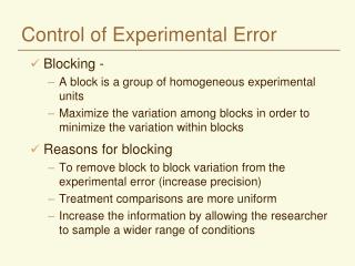
Control of Experimental Error • Blocking - • A block is a group of homogeneous experimental units • Maximize the variation among blocks in order to minimize the variation within blocks • Reasons for blocking • To remove block to block variation from the experimental error (increase precision) • Treatment comparisons are more uniform • Increase the information by allowing the researcher to sample a wider range of conditions
A B D A A B D C C D B C C D B A B A D C B A D C Just replication Blocking Blocking • At least one replication is grouped in a homogeneous area
Criteria for blocking • Proximity or known patterns of variation in the field • gradients due to fertility, soil type • animals (experimental units) in a pen (block) • Time • planting, harvesting • Management of experimental tasks • individuals collecting data • runs in the laboratory • Physical characteristics • height, maturity • Natural groupings • branches (experimental units) on a tree (block)
Randomized Block Design • Experimental units are first classified into groups (or blocks) of plots that are as nearly alike as possible • Linear Model: Yij = + i + j + ij • = mean effect • βi = ith block effect • j = jth treatment effect • ij = treatment x block interaction, treated as error • Each treatment occurs in each block, the same number of times (usually once) • Also known as the Randomized Complete Block Design • RBD = RCB = RCBD • Minimize the variation within blocks - Maximize the variation between blocks
Randomized Block Design Other ways to minimize variation within blocks: • Field operations should be completed in one block before moving to another • If plot management or data collection is handled by more than one person, assign each to a different block
Advantages of the RBD • Can remove site variation from experimental error and thus increase precision • When an operation cannot be completed on all plots at one time, can be used to remove variation between runs • By placing blocks under different conditions, it can broaden the scope of the trial • Can accommodate any number of treatments and any number of blocks, but each treatment must be replicated the same number of times in each block • Statistical analysis is fairly simple
Disadvantages of the RBD • Missing data can cause some difficulty in the analysis • Assignment of treatments by mistake to the wrong block can lead to problems in the analysis • If there is more than one source of unwanted variation, the design is less efficient • If the plots are uniform, then RBD is less efficient than CRD • As treatment or entry numbers increase, more heterogeneous area is introduced and effective blocking becomes more difficult. Split plot or lattice designs may be better suited.
Uses of the RBD • When you have one source of unwanted variation • Estimates the amount of variation due to the blocking factor
Randomization in an RBD • Each treatment occurs once in each block • Assign treatments at random to plots within each block • Use a different randomization for each block
Analysis of the RBD • Construct a two-way table of the means and deviations for each block and each treatment level • Compute the ANOVA table • Conduct significance tests • Calculate means and standard errors • Compute additional statistics if appropriate: • Confidence intervals • Comparisons of means • CV
The RBD ANOVA Source df SS MS F Total rt-1 SSTot = Block r-1 SSB = MSB = MSB/MSE SSB/(r-1) Treatment t-1 SST = MST = MST/MSE SST/(t-1) Error (r-1)(t-1) SSE = MSE = SSTot-SSB-SSTSSE/(r-1)(t-1) MSE is the divisor for all F ratios
Means and Standard Errors Standard Error of a treatment mean Confidence interval estimate Standard Error of a difference Confidence interval estimate on a difference t to test difference between two means
Numerical Example • Test the effect of different sources of nitrogen on the yield of barley: • 5 sources and a control • Wanted to apply the results over a wide range of conditions so the trial was conducted on four types of soil • Soil type is the blocking factor • Located six plots at random on each of the four soil types
Source (NH4)2SO4 NH4NO3 CO(NH2)2 Ca(NO3)2 NaNO3 Control Mean 36.25 32.38 29.42 31.02 30.70 25.35 ANOVA Source df SS MS F Total 23 492.36 Soils (Block) 3 192.56 64.19 21.61** Fertilizer (Trt) 5 255.28 51.06 17.19** Error 15 44.52 2.97 Standard error of a treatment mean = 0.86 CV = 5.6% Standard error of a difference between two treatment means = 1.22
Confidence Interval Estimates 34.41 30.54 29.19 28.86 27.59 23.51 36.25 32.38 31.02 30.70 29.42 25.35 38.09 34.21 32.86 32.54 31.26 27.19
Report of Analysis • Differences among sources of nitrogen were highly significant • Ammonium sulfate (NH4)2SO4 produced the highest mean yield and CO(NH2)2 produced the lowest • When no nitrogen was added, the yield was only 25.35 kg/plot • Blocking on soil type was effective as evidenced by: • large F for Soils (Blocks) • small coefficient of variation (5.6%) for the trial
Is This Experiment Valid? Full Irrigation Irrigated Pre-Plant No Irrigation
Missing Plots • If only one plot is missing, you can use the following formula: Yij = ( rBi + tTj - G)/[(r-1)(t-1)] • Where: • Bi= sum of remaining observations in the ith block • Tj = sum of remaining observations in the jth treatment • G = grand total of the available observations • t, r= number of treatments, blocks, respectively • Total and error df must be reduced by 1 • Used only to obtain a valid ANOVA • No change in Error SS • SS for treatments may be biased upwards
^ Yij = ( rBi + tTj - G)/[(r-1)(t-1)] Two or Three Missing Plots • Estimate all but one of the missing values and use the formula • Use this value and all but one of the remaining guessed values and calculate again; continue in this manner until you have resolved all missing plots • You lose one error degree of freedom for each substituted value • Better approach: Let SAS account for missing values • Use a procedure that can accommodate missing values (PROC GLM, PROC MIXED) • Use adjusted means (LSMEANS) rather than MEANS • degrees of freedom are subtracted automatically for each missing observation
Relative Efficiency • A way to measure the efficiency of RBD vs CRD RE = [(r-1)MSB + r(t-1)MSE]/(rt-1)MSE Estimated Error for a CRD Observed Error for RBD • r, t = number of blocks, treatments in the RBD • MSB, MSE = block, error mean squares from the RBD • If RE > 1, RBD was more efficient • (RE - 1)100 = % increase in efficiency • r(RE) = number of replications that would be required in the CRD to obtain the same level of precision