Download
1 / 24
240 likes | 306 Views
Hash Tables With Finite Buckets Are Less Resistant to Deletions. Yossi Kanizo (Technion, Israel). Joint work with David Hay (Columbia U. and Hebrew U.) and Isaac Keslassy ( Technion ). Hash Tables for Networking Devices.

E N D
Hash Tables With Finite BucketsAre Less Resistant to Deletions Yossi Kanizo (Technion, Israel) Joint work with David Hay (Columbia U. and Hebrew U.) and Isaac Keslassy(Technion)
Hash Tables for Networking Devices • Hash tables and hash-based structures are often used in high-speed devices • Heavy-hitter flow identification • Flow state keeping • Flow counter management • Virus signature scanning • IP address lookup algorithms • In many applications elements are also deleted (a.k.a. dynamic hash tables)
Dynamic vs. Static • Dynamic hash tables are harder to model than the static ones, that is, insertions only [Kirsch et al.] • Past studies show same asymptotic behavior with infinite buckets(insertions only vs. alternations) • traditional hashing using linked lists – maximum bucket size of approx. log n / log log n[Gonnet, 1981] • d-random, d-left schemes – maximum bucket size of log log n / log 2+O(1) [Azar et al.,1994; Vöcking, 1999] • Using the static model seems natural.
High-Speed Hardware 6 h 7 3 1 5 2 8 9 4 Memory CAM 1 2 3 4 5 6 7 8 9 • Bucket is a memory word that contains h elements • E.g.: 128-bit memory word h=4 elements of 32 bits • Assumption: Access cost (read & write word) = 1 cycle • Enable overflows: after d memory accesses → overflow list • Can be stored in expensive CAM • Otherwise, overflow elements = lost elements • Overflow fraction =
Degradation with Finite Buckets Remove 1 • Finite buckets are used. • Degradation in performance Element “2” is not stored although its corresponding bucket is empty 2 1 H(2) = 3 H(1) = 3 2 1 1 1 2 3 4 1 2 3 4 Finite Infinite
Degradation with Finite Buckets • What we had is • Insert element “1” • Insert element “2” • Remove element “1” • Equivalent to only inserting element “2” in the static case 2 2 1 2 3 4 1 2 3 4 Finite Infinite
Simulations [h=1, load=n/(mh)=1, d = 2]
Comparing Static and Dynamic • Static setting: insertions only • n = number of elements • m = number of buckets • Dynamic setting: alternations between element insertions and deletions of randomly chosen elements. • fixed load of c = n / (mh) • Fair comparison • Given an average number of memory accesses a, minimize overflow fraction .
Why We Care about Average Number of Memory Accesses? • On-chip memory: memory accesses power consumption • Off-chip memory: memory accesses lost on/off-chip pin capacity • Datacenters: memory accesses network & server load • Parallelism does not help reduce these costs • d serial or parallel memory accesses have same cost
From Discrete to Fluid Model • Discrete model • Models the system accurately but induces complex interactions between the elements • Approximation using a fluid model • Based on differential equations with an infinite number of elements and buckets. • Elements stay in the system for exponentially-distributed duration of average 1. • Bucket departure rate is proportional to its occupancy. • Upon departure, a new element arrives. • arrival rate is constant (fixed load in the system). • Assuming uniformly distributed hash functions, bucket arrival rate is n / m = ch
Main Results Case Study: Single choice hashing scheme Lower bound on overflow fraction Mitigating the degradation in performance.
Case Study: Analysis of Single Choice Hashing Scheme 1/m·(1-1/n) 1/m·(1-2/n) 1/m·(1-3/n) 1/m·(1-h/n) … (1-1/m) ·1/n (1-1/m) ·2/n (1-1/m) ·3/n h/n 1 2 h 0 • Departure rate is proportional to bucket occupancy; arrival rate is constant • We show that (limit of) discrete Markov chain fluid model • Intuition: No dependency between the buckets because of the single choice. No “complex interaction” • Bucket occupancy distribution is • The Overflow fraction is (Erlang-B formula)
Case Study: Numerical Example • For bucket size h=1, we get: g =c/(1 + c). • In case of 100% load (c=1): • dynamic: 50%. • static: 36.79%. [Kanizo et al., INFOCOM 2009] • In case of 10% load (c=0.1): • dynamic: 9.1%. • static: 4.84%. • As load 0, dynamic systems has twice the overflow fraction of static systems.
Main Results Case Study: Single choice hashing scheme Lower bound on overflow fraction Mitigating the degradation in performance.
Overflow Lower Bound • Objective: given any online scheme with average a, find lower-bound on the overflow fraction . • We use the fluid model • Elements arrival rate is ch = n / m. • Hashing rate per element is a. • In the best case, all memory accesses are used to store elements.
Overflow Lower Bound • Overflow lower bound ofwhere r = ach. • Also holds for non-uniformly distributed hash functions (under some constraints).
Numerical Example • For bucket size h=1, lower bound of 1-a/(1+ac). • 100% load (c=1) implies lower bound of 1/(1+a). • To get an overflow fraction of 1%, one needs at least 99 memory accesses per element. • Infeasible for high-speed networking devices • Compared to a tight upper bound of e-a in the static case. [Kanizo et al., INFOCOM 2009] • need ~4.6 memory accesses.
The Lower Bound is Tight • Single choice hashing scheme • Optimal for a = 1 • Multiple choice: Try to insert each element greedily until either inserted or d trials. • Optimal for larger number of memory accesses, depending on system parameters. • Example: • h = 4, c = 1, d = 4 • Multiple choice is optimal for a 2.19 .
Main Results Case Study: Single choice hashing scheme Lower bound on overflow fraction Mitigating the degradation in performance.
Moving Back Elements • Recall the example from the beginning Element “2” is not stored although its corresponding bucket is empty 2 1 2 3 4 1 2 3 4 Finite Infinite
Moving Back Elements • Overflow elements are stored in CAM. • Moving back elements from the CAM to the buckets. • We cannot check upon a deletion every element in the CAM. • Store the hash values along with the elements in the CAM. • Upon departure check if an element can be moved back. • Can be combined with any hashing insertion scheme.
Evaluation • Single choice hashing scheme • Performance is exactly as in the static case. • Multiple choice hashing scheme • Performance is better than the static case, albeit with more memory accesses. [h=4, d=1]
Wrap-up • Initial simulation results show degradation in performance. • We found lower and upper bounds on the achievable overflow fraction. • We compared it with upper bounds of the static case. • Mitigating the degradation in performance. • Also in the paper • Simulations with synthetic data • Other dynamic models • Trace-driven simulations