Bootstrap Test for Pairs of Means of a Non-Normal Population – small samples

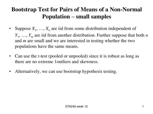
1. Bootstrap Test for Pairs of Means of a Non-Normal Population – small samples • Suppose X1, …, Xn are iid from some distribution independent of Y1, …, Ym are iid from another distribution. Further suppose that both n and m are small and we are interested in testing whether the two populations have the same means. • Can use the t-test (pooled or unpooled) since it is robust as long as there are no extreme 1outliers and skewness. • Alternatively, we can use bootstrap hypothesis testing. STA248 week 12

2. Bootstrap Hypothesis Testing - Introduction • Suppose X1, …, Xn is a random sample of size n, independent from another random sample Y1, …, Ym of size m.and we wish to test vs . • As a test statistics we will use . • The P-values of this test is . • We want the bootstrap estimate of this P-value. STA248 week 12

3. Bootstrap Test Procedure • To obtain the bootstrap estimate of the P-value we need to generate samples with H0 true. • One way of doing this (assuming X and Y have same distribution) is to combine 2 samples into 1 of size n+m. • Then re-sample with replacement from this combined sample such that each re-sampling has two groups … • For each bootstrap sample calculate the bootstrap estimate of the test statistics , j = 1, …, B. • The bootstrap estimate of the P-value is…. STA248 week 12

4. Example STA248 week 12

5. Data Collection There are three main methods for collecting data. Observational studies Sample survey Planned / designed experiments These methods differ in the strength of conclusion that can be drawn. STA248 week 12 5

6. Observational Studies In some cases, a study may be undertaken retrospectively. In observational studies we simply collect information about variables of interest without applying any intervention or controlling for any factors. When factors are not controlled we are not able to infer a cause- effect relationship. Other problems with observation studies are: Confounding – can’t separate effect of one variable from another. Lack of generalization. STA248 week 12 6

7. Sample Surveys Sample surveys are observational in nature. Surveys require existence of physically real population. Data is collected on a random sample from the target population. Survey design includes selection of sample so it is representative of the population as a whole. Use statistics to make inference about entire population. Confounding is still a problem. However, the results can be generalized to the population. Cause of any observed differences cannot be determined. To allow generalization and to avoid bias – sample must be chosen randomly e.g., SRS. STA248 week 12 7

8. Planned / Designed Experiments There are few key features of designed experiments that distinguish it from any other type of study. Independent variables of interest are carefully controlled by the experimenter in order to determine their effect on a response (dependent) variable. Researcher randomly assign a treatment to the subjects or experimental units. Control of independent variables and randomization make it possible to infer cause and effect relationship. Use of replication – multiple observation per treatment. Replication allows measurement of variability. STA248 week 12 8

9. Treatments are sometimes called predictor variables and sometimes called “factors”. • The values of a factor are its “levels”. • A design is balanced if each treatment has the same number of experimental units. • Problem: can’t always carry out an experiment. STA248 week 10

10. Randomization • The use of randomization to allocate treatments to experimental units (or vice versa) is the key element of well-designed experiment. • Random allocation tends to produce subgroups which are comparable with respect to the variables known to influence the response. • Randomization ensures that no bias is introduced in allocation of treatments to experimental units. • Randomization reduces the possibility that factors not included in the design will be confounded with treatment. STA248 week 12

11. Cautions Regarding Experiments • “Effective sample size” – all statistical techniques we have learned assume observations are independent. If they are not but treated as if they were, get more power and smaller CI than you should. • “Fishing expedition” – if doing 100 tests at α = 0.05 significant level, expect 5 of 100 tests to show significant differences from H0 even when H0 is always true (type I errors). STA248 week 10

12. Controlling for Type I error • One widely use method for controlling for type I error uses Bonferoni Inequality…. • If Ai is the event that the ith test has a type I error, and typically P(Ai ) = α, then by Bonferoni Inequality we that: .. That is the probability of committing at least one type I error in k tests is at most kα. • Therefore, if use significant level of α/k for each individual test, then the “overall significant level” (P(at least 1 type I error)) is at most α. • The Bonferoni method is very conserevative. STA248 week 10

13. Analysis of Variance – Introduction • Generalization of the two sample t-procedures (with equal variances). • The objective in analysis of variance is to determine whether there are differences in means of more than 2 groups. • The statistical methodology for comparing several means is called analysis of variance, or simply ANOVA. • When studying the effect of one factor only on the response we use one-way ANOVA to analyze the data. • When studying the effect of two factors on the response we use two-way ANOVA. STA248 week 10

14. One-Way ANOVA model • The response variable Y is measured on each experimental unit in each treatment group. Measure Yij for the jth subject in the ith group. • The one-way ANOVA model is: Yij = μi + εij for i = 1, 2,…, k and j = 1, 2, …, ni. • μi is the unknown mean response for the ith group. • The εij are called “random errors” and are assumed to be i.i.d N(0, σ2). • The parameters of the model are the population means μ1, μ2,…, μk and the common standard deviation σ. • The objective of one-way ANOVA is to test whether the mean response in each treatment group is the same. • The null and alternative hypotheses are…. STA248 week 10

15. Derivation of Test Statistics STA248 week 10