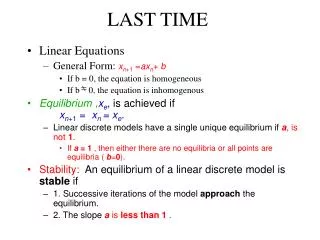
Linear Equations General Form: x n +1 = ax n + b If b = 0, the equation is homogeneous

1. LAST TIME • Linear Equations • General Form: xn+1 =axn+ b • If b = 0, the equation is homogeneous • If b 0, the equation is inhomogenous • Equilibrium ,xe, is achieved ifxn+1 = xn = xe. • Linear discrete models have a single unique equilibrium ifa, is not 1. • If a = 1 , then either there are no equilibria or all points are equilibria ( b=0). • Stability: An equilibrium of a linear discrete model is stableif • 1. Successive iterations of the model approach the equilibrium. • 2. The slopea is less than 1.

2. Systems of Linear Difference Equations • Sometimes you will be interested in two or more quantities that influence each others change from generation to generation.

3. Systems of Linear Difference Equations • Any system of linear first order difference equations can be converted to a single higher order system. • Increase order of one of the the equations, say the x equation 2. Eliminate yn+1

4. Systems of Linear Difference Equations • Any system of linear first order difference equations can be converted to a single higher order system. 3. Eliminate yn

5. Systems of Linear Difference Equations • Any system of linear first order difference equations can be converted to a single higher order system. This equation is 2nd order and requires two previous data points in order to determine the future value of x.

6. Finding the Solution • Look for solutions of the form: xn = Cn • Substitute into to get divide Cn by to obtain the Characteristic Equation

7. Finding the Solution • Solutions of the characteristic equation are called eigenvalues. • The properties of the eigenvalues uniquely determine the behavior of the solutions.

8. Principle of Superposition • For linear difference equations; if several different solutions are known, then any linear combination of the these solutions is again a solution. • Therefore the General Solution is: For real, distinct evals: For real, equal evals:

9. Dominant Eigenvalue • The dominant eigenvalue is the one with largest magnitude, ie the largest absolute value. • Because solutions to second order discrete equations are of the form: the dominant eigenvalue will have the strongest effect on the behavior of the solutions

10. Example

11. General Form of 2nd Order Discrete Equations • When b = 0, the solution for real, distinct eigenvalues is • When b = constant, the solution for real distinct eigenvalues is

12. Example

13. Qualitative Behavior of Linear,Discrete Equations • An mth order, linear discrete (difference) equation takes the form • The order, m, refers to the number of pervious generations that directly impact the value of x in a given generation • When coefficients are constants and bn = 0, the equation is homogeneous and solutions are linear combinations of the form: Cn

14. Qualitative Behavior of Linear,Discrete Equations • The number of basic solutions to a linear, discrete equation is determined by its order. • In general, an mth order equation has m basic solutions • The General Solution is a linear combination of the basic solutions (provided all values of the eigenvalues are distinct) • The eigenvalue with the largest magnitude will have the strongest effect on the behavior of the solutions

15. QUESTIONWhat if the Eigenvalues are Comnplex Numbers?

16. Complex Eigenvalues • The solution to a general characteristic polynomial can be a complex number. • A complex number, a + bi, is the point in the complex plane with coordinates (a,b). • Or equivalently, r a  b

17. Complex Eigenvalues • Complex e-vals occur in conjugate pairs, for example: • The general solution will then be: • What is (a +bi)n? • Recall Euler’s Formula a + bi = r(cos + isin) = rei a - bi = r(cos - isin) = re-i

18. Complex Eigenvalues • Using Euler’s Formula: (a +bi)n = (rein = rnein (a + bi)n = rn[cos(n + isin(n] • Similarly: (a - bi)n = (re-in = rne-in (a - bi)n = rn[cos(n - isin(n] Now substitute this into:

19. Complex Eigenvalues • So Therefore But this is a complex function …

20. Complex Eigenvalues • Define a real-valued solution by the superposition of the real and imaginary parts: • Therefore complex eigenvalues are associated with oscillatory solutions. The amplitude grows if r > 1, decreases if r < 1, and remains constant if r = 1. • Periodic solutions occur if  is a rational multiple of  and r = 1.

21. Example Solve: Characteristic Equation: Eigenvalues: Solution:

22. Failure of Programmed Cell Death and Differentiation as Causes of Tumors Some simple mathematical models

23. Hallmark Cancer Capabilities ?

24. Adenomatous polyps: Benign versus Malignant • Benign tumors are generally • composed of well-differentiated, slow growing cells; • enclosed in a fibrous capsule; • relatively innocuous, • Malignant tumors are generally • composed of poorly-differentiated, rapidly proliferating cells; • invasive and destructive to normal tissue; • metastatic, or capable of spreading to other sites of the body. Malignant gastric carcinoma

25. Cancer Stem Cell Hypothesis • Cancer stem cells have been identified in malignancies of the breast, brain, and blood and are believed to drive disease progression in these and possibly most cancers.

26. Hierarchal Cellular Systems • Stem Cells - the most naive • Progenitor Cells - precursors for mature cells • Differentiated Cells - carry out specific functions

27. Types of Division in Model • stem cell • differentiated cell Not considered! Symmetric self-renewal A new stem cell is added Asymmetric self-renewal Number of stem cells stays the same One differentiated cell is added Non-self-renewal division One stem cell is removed Two differentiated cells are added

28. Programmed Cell Death • A normal physiological response to cell stress, cell damage or conflicting cell division signals • Many cancers are hypothesized to arise from and are difficult to eradicate due to the failure to respond to apoptotic signals

29. Role of PCD in Tumorigenesis • Precise role is still unclear • Failure of PCD might give cells the equivalent of a replicative advantage • Failure to die is effectively the same as more rapid cell division • Failure of PCD may lead to an increase in the intrinsic mutation rate • Cells live longer and are exposed to more mutagens or acquire more spontaneous mutations

30. Failure of programmed cell death and differentiation as causes of tumors: Some simple mathematical modelsTomlinson and Bodmer, PNAS 1995

31. Basic Models of Tumor Growth • Assume tumor grows by increased cell division • A mutant cell population increases as mn+1 = 2mn mn = m02n • If mutants have a replicative advantage  mn = m0[2(1+w)]n, where w is the selective advantage of the mutant relative to a mean population of normal cells • All descendants of the original mutant cell population behave the same way

32. What happens when PCD is included? • This model doesn’t work • It cannot be assumed that cells behave as their parents do • A mutation occurring in a stem cell may have no effect until it is fully differentiated and about to undergo PCD • This cell may have divided many times • When cells differentiate and die a planned death, the effect of mutations will vary depending on when and where they occur • Timing is crucial!

33. Goal of the Study • Set up a simple mathematical model of tumorigenesis by failure of PCD and failure of differentiation • Use the model to demonstrate how tumor growth proceeds under these circumstances • Compare these results to the exponential growth predicted by increased cell division models

34. Definitions • P0 = a self-renewing population of stem cells • P1 = a population of cells at an intermediate differentiation state-- progenitor cells • P2 = a population of fully differentiated cells • P3 = the dead cell population P1 P0 P2 P3

35. Variables • Cn = number of stem cells after n divisions • Sn = number of intermediate cells after n divisions • Fn = number of fully differentiated cells after n divisions

36. Built in Assumptions • The number of cells in Pn (n = 0,1,2) depends on • The number of cells in Pn-1,for n = 1,2 • The rate of division of cells in Pn-1, for n = 1,2 • The probability that cells in Pn-1 differentiate into Pn cells rather than remain Pn-1 or die, for n = 1,2 • The rate of division of Pn cells, for n = 0,1 • The probability that cells in Pn differentiate into Pn+1 cells or die rather than remain in Pn, for n = 0,1

37. Parameters a1 = probability of stem cell (P0) death a2 = probability of stem cell (P0) differentiation a3 = probability of stem cell (P0) renewal b1 = probability of progenitor cell (P1) death b2 = probability of progenitor cell (P1) differentiation b3 = probability of progenitor cell (P1) renewal g = probability of mature cell (P2) death t0,t1, = time for one cell division to occur for stem cells (P0) and progenitor cells (P1) respectively.

38. Constraints Cells must do one of three things!

39. P0 P1 P2 P3 C S F D t0 t1 t2 Model Schematic Stage of Differentiation Number of Cells Generation Time

40. Normal Cell Division Model Equation At Equilibrium Stem Cell Population, C There is a unique probability of proliferation at which the stem cell population exactly renews itself. If 3 rises above or falls below 1/2, Cn Increase or decreases exponentially.

41. Normal Cell Division Model Equation Semi-differentiated (Progenitor) Cell Population, S At Equilibrium

42. Model Equation: Homogeneous Solution: Semi-differentiated (Progenitor) Cell Population, S Particular Solution: Let To Find:

43. Model Equation: General Solution: Semi-differentiated (Progenitor) Cell Population, S Apply Initial Condition: To Find:

44. At Equilibrium • Case 1: There is no realistic equilibrium point if • 23t0/t1 > 1 because when t1/t0 < 23 (ie when the • cell cycle time for P1 relative to P0 is less than twice the probability of renewal), then Se is negative • In this case: Sn increases exponentially • Case 2: There is no equilibrium if Cn is not in equilibrium • Sn behaves as Cn does Semi-differentiated (Progenitor) Cell Population, S

45. Normal Cell Division Model Equation At Equilibrium Fully-differentiated Cell Population, F • Case 1: When Cn and Sn are in equilibrium, so is Fn • Case 2: There is not equilibrium if Sn is not in equilibrium •  Fn behaves as Sn does

46. Model Predictions

47. Model Tissue Composition 1.2% 6.2% 92.6%

48. About These Results • Results illustrate the increased complexity of behavior that accompanies models that considers cell differentiation and PCD • If we restrain parameters so that the cell populations are in equilibrium, the limits for the stem cell population are restrictive, but restrictions weaken for the other cell populations • Now let’s analyze the case in which a mutation has altered the proportions of cells dying, differentiating or renewing themselves in order to determine the effects on tumorigenesis

49. Changes in the Probability of F-Cells Undergoing PCD,  • What happens if  changes by  where 0 <  +  < 1? • This mutation might have occurred in the P2 population itself and if so would not have had a large effect. • It is more likely that the mutation occurred in P0 or P1, but only has an effect on the P2 cells.

50. Probability of Death/Survival • is the probability of a fully differentiated cell dying • t2 is the time it for a takes a cell to die •  t0 t2is the probability that a mature cell dies in the time it take for a stem cell to divide. • A fully mature cell either lives or dies • The probability of survival is one minus the probability of death during the time it takes a stem cell to divide ie 1 -  t0 t2