Download
1 / 56
1.45k likes | 2.81k Views
Feature Extraction and Analysis (Shape Features). Disampaikan oleh : Nana Ramadijanti. Content. Introduction Feature Extraction Shape Features - Binary Object Features Feature Analysis Feature Vectors and Feature Spaces Distance and Similarity Measures. Introduction.

E N D
Feature Extraction and Analysis(Shape Features) Disampaikan oleh : Nana Ramadijanti
Content • Introduction • Feature Extraction • Shape Features - Binary Object Features • Feature Analysis • Feature Vectors and Feature Spaces • Distance and Similarity Measures
Introduction • The goal in image analysis is to extract useful information for solving application-based problems. • The first step to this is to reduce the amount of image data using methods that we have discussed before: • Image segmentation • Filtering in frequency domain
Introduction • The next step would be to extract features that are useful in solving computer imaging problems. • What features to be extracted are application dependent. • After the features have been extracted, then analysis can be done.
Shape Features • Depend on a silhouette (outline) of an image • All that is needed is a binary image
Binary Object Features • In order to extract object features, we need an image that has undergone image segmentation and any necessary morphological filtering. • This will provide us with a clearly defined object which can be labeled and processed independently.
Binary Object Features • After all the binary objects in the image are labeled, we can treat each object as a binary image. • The labeled object has a value of ‘1’ and everything else is ‘0’. • The labeling process goes as follows: • Define the desired connectivity. • Scan the image and label connected objects with the same symbol.
Binary Object Features • After we have labeled the objects, we have an image filled with object numbers. • This image is used to extract the features of interest. • Among the binary object features include area, center of area, axis of least second moment, perimeter, Euler number, projections, thinness ration and aspect ratio.
Binary Object Features • In order to extract those features for individual object, we need to create separate binary image for each of them. • We can achieve this by assigning 1 to pixels with the specified label and 0 elsewhere. • If after the labeling process we end up with 3 different labels, then we need to create 3 separate binary images for each object.
Binary Object Features – Area • The area of the ithobject is defined as follows: • The area Ai is measured in pixels and indicates the relative size of the object.
Binary Object Features – Area A1 = 7, A2 = 8, A3 = 7
Binary Object Features – Area(Matlab) • BW = imread('circles.png'); • imshow(BW); >> bwarea(BW) >> ans = 1.4187e+04
Binary Object Features – Center of Area • The center of area is defined as follows: • These correspond to the row and column coordinate of the center of the ith object.
Binary Object Features – Axis of Least Second Moment • The Axis of Least Second Moment is expressed as - the angle of the axis relatives to the vertical axis.
Binary Object Features – Axis of Least Second Moment • This assumes that the origin is as the center of area. • This feature provides information about the object’s orientation. • This axis corresponds to the line about which it takes the least amount of energy to spin an object.
Binary Object Features – Axis of Least Second Moment (in C) rcI = 0; rrI = 0; ccI = 0; for (r=0; r<height; r++) { for (c=0; c<width; c++) { shiftedRow = r – centerRow; shiftedCol = c – centerCol; rcI = rcI + (r * c * object_Image[r][c]); rrI = rrI + (r * r * object_Image[r][c]); ccI = ccI + (c * c * object_Image[r][c]); } } angle_in_radian = atan( 2 * rcI / (rrI - ccI) ) / 2; //Convert to degree angle_in_degree = angle_in_radian / * 180; //Convert to range 0 –180 relatives to vertical axis with counter-clock as +ve direction if (rrI – ccI < 0) angle_in_degree = angle_in_degree + 90; else if (rcI < 0) angle_in_degree = angle_in_degree +180;
Binary Object Features - Perimeter • The perimeter is defined as the total pixels that constitutes the edge of the object. • Perimeter can help us to locate the object in space and provide information about the shape of the object. • Perimeters can be found by counting the number of ‘1’ pixels that have ‘0’ pixels as neighbors.
Binary Object Features - Perimeter • Perimeter can also be found by applying an edge detector to the object, followed by counting the ‘1’ pixels. • The two methods above only give an estimate of the actual perimeter. • An improved estimate can be found by multiplying the results from either of the two methods by π/4.
Binary Object Features - Perimeter Perimeter=6 Perimeter=7 Perimeter=6
Binary Object Features – Thinness Ratio • The thinness ratio, T, can be calculated from perimeter and area. • The equation for thinness ratio is defined as follows:
Binary Object Features – Thinness Ratio • The thinness ratio is used as a measure of roundness. • It has a maximum value of 1, which corresponds to a circle. • As the object becomes thinner and thinner, the perimeter becomes larger relative to the area and the ratio decreases.
Binary Object Features - Thinness Ratio Compactness or Irregularity ratio T = 0.62 T = 1.4 T = 0.52 1/T = 1.6 1/T = 0.7 1/T = 1.9
Binary Object Features – Irregularity Ratio • The inverse of thinness ration is called compactness or irregularity ratio, 1/T. • This metric is used to determine the regularity of an object: • Regular objects have less vertices (branches) and hence, less perimeter compare to irregular object of the same area.
Binary Object Features – Aspect Ratio • The aspect ratio (also called elongation or eccentricity) is defined by the ratio of the bounding box of an object. • This can be found by scanning the image and finding the minimum and maximum values on the row and column where the object lies.
Binary Object Features – Aspect Ratio • The equation for aspect ratio is as follows: • It reveals how the object spread in both vertical and horizontal direction. • High aspect ratio indicates the object spread more towards horizontal direction.
Binary Object Features – Euler Number • Euler number is defined as the difference between the number of objects and the number of holes. • Euler number = num of object – number of holes • In the case of a single object, the Euler number indicates how many closed curves (holes) the object contains.
Binary Object Features – Euler Number • Euler number can be used in tasks such as optical character recognition (OCR).
Convexities Concavities Binary Object Features – Euler Number • Euler number can also be found using the number of convexities and concavities. • Euler number = number of convexities – number of concavities • This can be found by scanning the image for the following patterns:
Binary Object Features – Projection • The projection of a binary object, may provide useful information related to object’s shape. • It can be found by summing all the pixels along the rows or columns. • Summing the rows give horizontal projection. • Summing the columns give the vertical projection.
Binary Object Features – Projection • We can defined the horizontal projection hi(r) and vertical projection vi(c) as: • An example of projections is shown in the next slide:
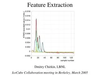
0 0 1 0 1 0 2 0 1 0 0 1 0 2 0 1 0 0 1 0 2 Integral proyeksi horisontal 1 1 1 1 1 1 6 0 0 0 0 1 0 1 0 0 0 0 1 0 1 1 3 2 1 6 1 Integral proyeksi vertikal Integral Proyeksi Fitur : 1 3 2 1 6 1 2 2 2 6 1 1
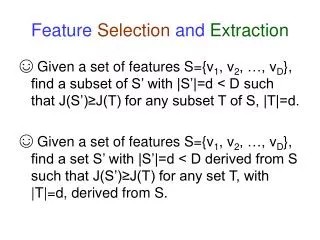
1 0 0 1 1 1 0 1 1 1 1 0 6 2 0 0 1 0 0 0 0 0 1 1 0 0 1 2 0 0 0 1 0 0 1 0 1 0 0 0 2 1 Integral proyeksi vertikal Integral proyeksi vertikal 0 1 1 0 1 1 0 1 1 0 0 1 6 1 0 0 1 0 0 0 0 0 1 0 0 0 1 1 0 1 0 0 0 0 0 0 1 0 0 0 1 1 2 1 2 3 2 2 2 1 2 6 1 1 Integral proyeksi horisontal Integral proyeksi horisontal Membandingkan Fitur Gambar Angka Fitur angka 4: 1 3 2 1 6 1 2 2 2 6 1 1 Fitur Angka 7: 2 2 2 2 2 1 6 1 1 1 1 1 Nilai perbedaan= 1+1+0+1+4+0+4+1+1+5+0+0=18
0 0 1 1 1 1 1 1 1 1 0 0 4 4 1 1 0 0 0 0 0 0 0 0 1 1 2 2 1 0 1 0 1 0 1 0 0 1 0 1 2 4 Integral proyeksi horisontal Integral proyeksi horisontal 1 1 0 0 0 0 0 0 0 0 1 1 2 2 1 1 0 0 0 0 0 0 0 0 1 1 2 2 0 0 1 1 1 1 1 1 1 1 0 0 4 4 3 4 3 2 2 3 3 2 3 2 3 4 Integral proyeksi vertikal Integral proyeksi vertikal Membandingkan Fitur Gambar Angka Fitur angka 0: 4 2 2 2 2 4 4 2 2 2 2 4 Fitur Angka 8: 3 3 3 3 3 3 4 2 4 2 2 4 Nilai perbedaan= 1+1+1+1+1+1+0+0+2+0+0+0=7
Feature Analysis • Important to aid in feature selection process • Initially, features selected based on understanding of the problem and developer’s experience • FA then will examine carefully to see the most useful & put back through feedback loop • To define the mathematical tools – feature vectors, feature spaces, distance & similarity measurement
Feature Vectors • A feature vector is a method to represent an image or part of an image. • A feature vector is an n-dimensional vector that contains a set of values where each value represents a certain feature. • This vector can be used to classify an object, or provide us with condensed higher-level information regarding the image.
Feature Vector • Let us consider one example: We need to control a robotic gripper that picks parts from an assembly line and puts them into boxes (either box A or box B, depending on object type). In order to do this, we need to determine: 1) Where the object is 2) What type of object it is The first step would be to define the feature vector that will solve this problem.
Feature Vectors To determine where the object is: Use the area and the center area of the object, defined by (r,c). To determine the type of object: Use the perimeter of object. Therefore, the feature vector is: [area, r, c, perimeter]
Feature Vectors • In feature extraction process, we might need to compare two feature vectors. • The primary methods to do this are either to measure the difference between the two or to measure the similarity. • The difference can be measured using a distance measure in the n-dimensional space.
Feature Spaces • A mathematical abstraction which is also n-dimensional and is created for a visualization of feature vectors
2-dimensional space • Feature vectors of x1 and x2 and two classes represented by x and o. • Each x & o represents one sample in feature space defined by its values of x1 and x2
Distance & Similarity Measures • Feature vector is to present the object and will be used to classify it • To perform classification, need to compare two feature vectors • 2 primary methods – difference between two or similarity • Two vectors that are closely related will have small difference and large similarity
Distance Measures • Difference can be measured by distance measure in n-dimensional feature space; the bigger the distance – the greater the difference • Several metric measurement • Euclidean distance • Range-normalized Euclidean distance • City block or absolute value metric • Maximum value
Distance Measures • Euclidean distance is the most common metric for measuring the distance between two vectors. • Given two vectors A and B, where:
Distance Measures • The Euclidean distance is given by: • This measure may be biased as a result of the varying range on different components of the vector. • One component may range 1 to 5, another component may range 1 to 5000.
Ri is the range of the ith component. Distance Measures • A difference of 5 is significant on the first component, but insignificant on the second component. • This problem can be rectified by using range-normalized Euclidean distance:
Distance Measures • Another distance measure, called the city block or absolute value metric, is defined as follows: • This metric is computationally faster than the Euclidean distance but gives similar result.
Distance Measures • The city block distance can also be range-normalized to give a range-normalized city block distance metric, with Ri defined as before:
Distance Measures • The final distance metric considered here is the maximum value metric defined by: • The normalized version: