Download
1 / 29
290 likes | 531 Views
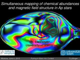
S imultaneous mapping of chemical abundances and magnetic field structure in Ap stars. Th. Lueftinger University of Vienna. Moskow, June 4, 2013 Putting A Stars into Context T.Lüftinger. Outline. Surface structures on Ap stars

E N D
Simultaneousmapping of chemicalabundances and magneticfieldstructure in Apstars Th. Lueftinger University of Vienna Moskow, June 4, 2013 Putting A Stars into Context T.Lüftinger
Outline • Surface structures on Ap stars • Doppler imaging and magnetic Doppler imaging (MDI) • Historical development • Principles, Technique • Ap - Examples • Bayesian Photometric imaging (BPI) • Conclusions Moskow, June 4, 2013 Putting A Stars into Context T.Lüftinger
Spots on Ap Stars • rotational axis OP • inclination angle i • observers line of sight: z-axis • axis of quasi-dipolar magnetic field OM • inclined by angle βto OP • -> vertical abundance gradients (see talk by T. Ryabchikova) • -> horizontal abundance gradients Moskow, June 4, 2013 Putting A Stars into Context T.Lüftinger
The History of (Magnetic) Doppler Imaging • First solution for determining surface anomalies from observed spectra presented by Deutsch (1958): equ. widths and magnetic potential developed into spherical harmonics, and Laplace coefficients of these expansions related to Fourier coefficients of the observed curves – ingenious, but limited -informations of line profile variations could not be used, surface resolution poor • Pyper (1969), Rice (1970) and Falk & Wehlau (1974) changed from using line strength variations to working with variations of the line profile shape -> contains much more information - Doppler Imaging as we know it today, can be ascribed to their work. • During mid 1970‘s Russian astronomers (Goncharsky et al., 1977), for the first time solved the inverse problem - mathematical equations relating inhomogeneities of temperature or abundance on a stellar surface to time series of observed line profiles - using the Tikhonov regularization method (Tikhonov, 1963) Moskow, June 4, 2013 Putting A Stars into Context T.Lüftinger
The History of (Magnetic) Doppler Imaging • Application of the according computer codes and remarkable increase in data quality in the following years notably increased the potential of this technique • Collaboration between Rice, Wehlau and Khokhlova: mapping of several Ap stars (first results for ε UMa in 1981 (Rice, Wehlau, Khokhlova & Piskunov, 1981) • Vogt, Penrod and Hatzes (Vogt & Penrod, 1983) extended Doppler Imaging work to cool stars and presented (Vogt, Penrod and Hatzes, 1987) a new inversion technique based on the Maximum Entropy Regularization Method (MEMSYS). • In the following years, groups around Piskunov, Rice, and Wehlau, in collaboration with Tuominen and Strassmeier, & around Vogt, Penrod, and Hatzes refine DI programs and extend their application. Astronomers like Cameron (1990), Brown et al. (1991), or Kürster (1993) contribute with significant Doppler Imaging work or publish new computer codes. • Important step in the beginning of the 1990‘s: Magnetic/Zeeman Doppler Imaging (ZDI), which involves Stokes parameters I, Q, U, and V in the analysis presented by Semel and Donati, in collaboration with Brown and Rees (Brown, Donati, Rees, Semel, 1991) and independently by Piskunov and Rice (1993)
Different Codes Spectroscopy, Spectropolarimetry Cool stars: DOTS (Collier Cameron 1995, 1997), brightness, modified version extended towards ZDI TEMPMAP (Rice & Strassmeier 2000) – temperature iMAP (Kopf, Caroll et al. 2009) magnetic-imaging code of Brown et al. (1991), Donati et al. (2001, 2006), Hussain et al. (2010), Petit et al. (2004) – surface field, brightness, accretion powered excess; INVERS13 (Kochukhov & Piskunov 2009, Rosén & Kochukhov, 2012) Hot stars: INVERS7, INVERS8, INVERS10, INVERS12, INVERS13 (Piskunov & Kochukhov 2002; Kochukhov & Piskunov 2002) magnetic-imaging code of Brown et al. (1991), Donati et al. (2001, 2006), Petit et al. 2011 – surface field, abundances (separately); Moskow, June 4, 2013 Putting A Stars into Context T.Lüftinger
Mapping Ap stars – The beginnings HD 124224, Si equivalent widths Goncharsky et al., 1977 CU Vir Hatzes, 1996 Moskow, June 4, 2013 Putting A Stars into Context T.Lüftinger
(Magnetic) Doppler Imaging - Principles Moskow, June 4, 2013 Putting A Stars into Context T.Lüftinger
(Magnetic) Doppler Imaging – Theory INVERS10 (N. Piskunov & O. Kochukhov, 2002) 1. Calculation of local synthetic Stokes profiles for n surface elements MRT solved for each visible surface element on each iteration 2. Disk integration of the Stokes profiles, contribution of each element depending on: 3. Regularization: Tikhonov, ME, Multipolar regularization 4. Minimization of observed and calulcated profiles Moskow, June 4, 2013 Putting A Stars into Context T.Lüftinger
The oblique rotator Rotational Modulation of Stokes Profiles Bd = 10 kG, b=45o ; i = 90o, v sini = 10 kms-1 Moskow, June 4, 2013 Putting A Stars into Context T.Lüftinger
Spectroplarimeters • SemelPol (AAT) • SOFIN (NOT) in polarimetric mode • ESPaDOnS (CFHT) • NARVAL (TBL) • HARPSpol (3.6-m telescope, ESO, La Silla)
Spectroplarimeters • SemelPol (AAT) • SOFIN (NOT) in polarimetric mode • ESPaDOnS (CFHT) • NARVAL (TBL) • HARPSpol (3.6-m telescope, ESO, La Silla)
Spectroplarimeters • SemelPol (AAT) • SOFIN (NOT) • ESPaDOnS (CFHT) • NARVAL (TBL) • HARPSpol (ESO 3.6-m) Moskow, June 4, 2013 Putting A Stars into Context T.Lüftinger
Spectroplarimeters SemelPol (AAT) SOFIN (NOT) in polarimetric mode ESPaDOnS (CFHT) NARVAL (TBL) HARPSpol (3.6-m telescope, ESO, La Silla)
Mapping Ap stars: 53 Cam intensely studied Ap star, e.g.: Landstreet 1988, Bagnulo et al. 2001 Kochukhov et al. 2004
HR 3831 correlation with magnetic field geometry no obvious correlation • ‘typical‘ (‘usually‘ expected) Ap-star spot structure of iron peak elements distributed around magnetic equator and REE at the poles of a dipolar field not confirmed • actually only a few elements (e.g. Li, O, Eu) show a well defined spot or ring correleated with the dipolar field component - most other not (obviously) do • are those preferrentially sensitive to horizontal magnetic field component (complex topology as seen in Stokes IQUV analysis)? diversity in distribution of heavy elements Kochukhov et al. 2004
Mapping Ap stars: α2 CVn Inversions based on full Stokes parameter sets IQUV reveal complex fields surface magnetic field derived from Stokes IQUV (Fe II and Cr II, contours of equal magnetic field strength plotted every 0.5 kG) same as above, but 10 times larger Tikhonov regularization surface magnetic field derived using Stokes I and V with multipolar regularization* Kochukhov & Wade 2010 * difference between the ‚current‘ solution and the best multipolar fit to this solution
Observations in Stokes IV HR1217 = HD24712 16 different chemical species plus magnetic field geometry Lüftinger et al. 2010 • group of elements with maximum abundance around the phase where the positive magnetic pole is visible (all REE plus Ca, Co, and Y) • the other group is enhanced where the magnetic equatorial region dominates the visible surface (e.g. Cr, Ti, Mg, Fe, Ni, Sc)
Mapping Ap stars: HD 24712 • we observe shifts of maximum/minimum abundance regions for various elements (chemically ‘stratified tail’) Elements mapped and theirabundancerange Lüftinger et al. 2010 what could this tell us about diffusion properties for the different spezies
Observations in Stokes IQUV The closer we look, the more complex the fields seem to be The closer we look, the more complex the fields seem to be Rusomarov et al., in prep. Moskow, June 4, 2013 Putting A Stars into Context T.Lüftinger
Cu Vir: MDI Magnetic field geometry based on LSD profiles Lüftinger, Kochukhov et al. and the MiMeS Collaboration in prep. Moskow, June 4, 2013 Putting A Stars into Context T.Lüftinger
MDI: τ Sco Donati et al., 2006, analogues HD66665 and HD63425 discussed by Petit et al., 2011 closed (left two panels, ph: 0.25, 0.83) and open field lines (right panel ph: 0.83), extrapolated from the photospheric map on the left B0.2 V magnetic star rotational modulation stable on timescales of decades, with Prot ≃ 41.03 d surface magnetic topology unusually complex, magnetic topology reconstructed more likely to be of fossil origin (≠ various dynamo mechanisms proposed in the literature for hot, massive stars) -> could indicate, that very hot magnetic stars represent a high-mass extension of the classical Ap/Bp phenomenon, no chemical peculiarities -> probably related to their strong winds, which prevent photospheric element stratification to build up
Bayesian Photometric Imaging (BPI) MOST! Upcoming: PLATO, BRITE-C CoRoT – ‘COnvection, ROtation and planetary Transits’ Kepler – A Search for Habitable Planets, Asteroseismology within KASC lightcurves to determine spot locations on the surface using a Photometric Imaging method based on Bayesian parameter estimation (H.-E. Fröhlich)
‘Alltogether’ Spectropolarimetry, Photometry, Spectroscopy Lüftinger, Fröhlich et al. 2010 Bd = 10 kG, b=45o ; i = 90o, v sini = 10 kms-1 chemical patches give rise to bright spots
Conclusions • Pronounced diversity of spot structures • Indication of complex fields from linear Stokes parameters • Bayesian Photometric imaging as an asset • (M)DI of Ap stars help to successfully explain their photometric variations (see talk of Krticka et al. and Krticka et al., 2012, Shulyak et al. 2010) • -> continue investigations to increase statistics an find similarities THANK YOU! Moskow, June 4, 2013 Putting A Stars into Context T.Lüftinger
Bayesian Photometric Imaging (BPI) e.g. two spots on a stellar surface ➛ nine free parameters: two periods, two epochs, two latitudes, two spot areas, and the star’s inclination splitting the nine-parameter problem (unsolvable) into two parts: 1. finding the two periods and epochs (times of minimal light) - AMOEBA 2. scanning the remaining parameter space - FROEHLICH 3. Bayesian data analysis: the whole likelihood mountain is considered, integrating all parameters, except one, we obtain the marginal probability distribution of this parameter HD 50773 ➛ results suggest four circular bright spots Moskow, June 4, 2013 Putting A Stars into Context T.Lüftinger
(Magnetic) Doppler Imaging – theory 2. Disk integration of the Stokes profiles, contribution of each element depending on: • Doppler shift due to stellar rotation • the projected area of a zone • the limb angle stellar and observer's coordinate system P: stellar pole: longitude CP: rotational axis : phase angle B: magnetic vector : azimuth angle Moskow, June 4, 2013 Putting A Stars into Context T.Lüftinger
(Magnetic) Doppler Imaging – theory 3. Regularization: DI and MDI (in cases without linear Stokes parameters) ill posed problem -> need ‘penalty funtion’: Ψ =χ2(Z,B) + Λ1R1(Z) + Λ2r2(B) B, Z: magnetic distributions and surface abundance R1 Tikhonov regularization functional R2 Tikhonov functional for the magnetic field Λ’s represent the corresponding regularization parameters In case of Stokes I and V mapping: +Λ3 R3(B) 4. Minimization: Marquardt-Levenberg method (Bevington & Robinson (1992) gradient search + linearizing the fitting function (rapid convergence close to the minimum) Moskow, June 4, 2013 Putting A Stars into Context T.Lüftinger