BASIC FEASIBLE SOLUTIONS
BASIC FEASIBLE SOLUTIONS. CONTENTS Polyhedral Sets and Polytopes Basic Feasible Solutions and Polytopes Reference: Chapters 2 and 3 in BJS book. Hyperplanes. A hyperplane in E n generalizes the notion of a straight line in E 2 and the notion of a plane in E 3 .

BASIC FEASIBLE SOLUTIONS
E N D
Presentation Transcript
BASIC FEASIBLE SOLUTIONS CONTENTS • Polyhedral Sets and Polytopes • Basic Feasible Solutions and Polytopes Reference: Chapters 2 and 3 in BJS book.
Hyperplanes A hyperplane in En generalizes the notion of a straight line in E2 and the notion of a plane in E3. A hyperplane H in En is a set of the form {x:px=k} where p is a nonzero vector in En and k is a scalar. If x0 H, then px0 = k, and for any other point x H, px = k. Hence, p(x – x0) = 0. Both hyperplanes and halfspaces are convex sets. Why?
d x0 Rays A ray is a collection of points of the form {x0 + d: 0}, where d is a nonzero vector. A convex cone C is a convex set with the additional property that x C for each x C and for each 0.
Polyhedron A hyperplane divides En into two regions, called halfspaces: S1 = {x: px k} S2 = {x: px k} A polyhedral set or a polyhedron is the intersection of a finite number of halfspaces. A bounded polyhedral set is called a polytope.
Polyhedral Sets Consider the polyhedral set defined by the following inequalities: -2x1 + x2 4 x1 + x2 3 x1 2 x1 0 x2 0 A polyhedral set can be represented by the set {x: Ax b} where A is an mxn matrix.
An Important Theorem Theorem: For any polytope S, every solution x can be represented by a convex combinations of the extreme points of the polytope. Let x1, x2, x3, … , xk denote the extreme points of a polytope S. Then, for any x S, there exist 1, 2, 3,.., k x = 1x1 + 2x2 + 3x3 + …. + kxk, where
Another Important Theorem Consider the following linear programming problem: Minimize cx subject to Ax = b x 0 Let x1, x2, x3, … , xk be the extreme points of the constraint set S. This linear program can be transformed into the following linear program: Minimize subject to 1, 2, 3, … , k 0 How to solve this linear program?
Another Important Theorem (contd.) Theorem. If a linear programming problem has a bounded feasible solution space, then there must exist an optimal extreme point solution. Is every optimal solution of a linear programming problem an extreme point solution? It can be shown that extreme point solutions correspond to basic feasible solutions (BFS) which are defined algebraically.
Standard Form of a Linear Program Condition 1: All right-hand side coefficients in the constraints are nonnegative. Condition 2 : All constraints are in the equality form. Condition 3 : All variables must take nonnegative values. Maximize c1x1 + c2x2 + c3x3 + …. + cnxn subject to a11x1 + a12x2 + a13x3 + …. + a1nxn= b1 a21x1 + a22x2 + a23x3 + …. + a2nxn= b2 : : am1x1 + am2x2 + am3x3 + …. + amnxn= bm x1, x2, x3 , …., xn 0
Restoring Condition 1 Condition 1: All right-hand side coefficients in the constraints are nonnegative. Constraint: 2x1 - 3x2 + x3 - 10 Alternative constraint: -2x1 + 3x2 - x3 10
Restoring Condition 2 Condition 2 : All constraints are in the equality form. max z = 4x1+ 3x2 max z = 4x1+ 3x2 s.t. x1 + x2 40 x1 + x2 + s1= 40 2x1+ x2 60 2x1+ x2 + s2= 60 x1, x2 0 x1, x2, s1, s2 0 max z = 4x1+ 3x2 max z = 4x1+ 3x2 s.t. x1 + x2 40 x1 + x2 - e1= 40 2x1+ x2 60 2x1+ x2 - e2= 60 x1, x2 0 x1, x2, e1, e2 0 si= Slack variables ei = Surplus variables
Restoring Condition 3 Condition 3 : All variables must take nonnegative values. max z = 30x1 - 4x2 + 8x3 s.t. 5x1 - x2 + x3 30 x1 5 x1 0, x2 unrestricted, x3 0 Variable transformation: x2 = , = - x3 max z = 30x1 - 4( ) - 8 s.t. 5x1 - - 30 x1 5 x1, , , 0
Basic Feasible Solutions Consider the linear program with the constraints: Ax=b and x 0 Where A is an mxn matrix and b is an m vector. Let rank (A) = m. Let A= [B,N] where B is an m x m invertible matrix, and N is an m x (n-m) matrix. Then the solution of the system BxB = b is a basic solution of the linear program.
Basic Feasible Solutions (contd.) Alternatively, the solution x = [xB, xN] xB = B-1 b xN= 0 is the basic solutions of the system. If xB 0, then x is called a basic feasible solution (BFS) of the system. A basic feasible solution x is called a degenerate basic feasible solution if some component of xB is zero. B is called the basis matrix. Variables in xB are called basic variables. Variables in xN are called nonbasic variables.
Example 1 Consider a polyhedral set: Standard form: x1 + x2 6x1 + x2 + x3 = 6 x2 3 x2 + x4 = 3 x1 , x2 0 x1 , x2 , x3 ,x4 0 Constraint Matrix: A= [a1, a2, a3, a4] =
Example 1 (contd.) The solution space:
Example 1 (contd.) B = [a1,a2] = xB = xN =
Example 1 (contd.) B = [a1,a4] = xB = xN =
Example 1 (contd.) B = [a2,a3] = xB = xN =
Example 1 (contd.) B = [a2,a4] = xB = xN =
Example 1 (contd.) B = [a3,a4] = xB = xN =
Example 1 (contd.) Have we considered all the basic solutions? How many basic solutions there are? How many basic feasible solutions there are?
Example 1 (contd.) Four Basic Feasible Solutions:
Basic Feasible Solutions The possible number of basic feasible solutions is bounded by the number of ways of extracting m columns out of n columns. The maximum number of BFS =
Example 2 Consider a polyhedral set: Standard form: x1 + x2 6x1 + x2 + x3 = 6 x2 3 x2 + x4 = 3 x1 + 2x2 9x1 + 2x2 + x5 = 9 x1 , x2 0 x1 , x2 , x3 ,x4, x5 0 Constraint Matrix: A= [a1, a2, a3, a4] =
Example 2 (contd.) Feasible Solution Space:
Example 2 (contd.) B = [a1, a2, a3]; xB = xN = B = [a1, a2, a4]; xB = xN = B = [a1, a2, a5]; xB = xN = Observe that several basis correspond to the same basic feasible solution. Also observe that the basic feasible solution must be degenerate for it to happen.
Summary: Basic and Basic Feasible Solutions • Identify m linearly independent (basic) variables (BV). • Set the remaining n - m (nonbasic) variables to zero value (NBV). • Solve the equations Ax = b in terms of the basic variables. (Observe that there is a unique solution.) • The resulting solution is a basic solution (BS). • A basic solution is a basic feasible solution (BFS) if xj 0 for each j = 1, 2, … , N. • There are at most n!/(n-m)!m! BFS. Hence there are finite number of BFS.
Adjacent Basic Feasible Solutions For any LP with m constraints, two basic feasible solutions are said to be adjacent if their sets of basic variables have m-1 basic variables in common. Basic Feasible Solution: (x1, x2, x3, x4) Adjacent Basic Feasible Solutions: (x1, x2, x3, x5) (x1, x2, x6, x4) (x1, x7, x3, x4) (x8, x2, x3, x4)