Download
1 / 21
210 likes | 228 Views
This talk explores the relationship between instability and indexability in nearest neighbor problems in high dimensionality. It analyzes workloads, discusses the breakdown of nearest neighbor processing techniques, and examines scenarios where these techniques may perform well. The talk concludes with suggestions for future work, including examining contrast in mapping similarity problems and finding indexing structures for high contrast situations.

E N D
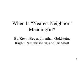
When Is “Nearest Neighbor” Meaningful? By Kevin Beyer, Jonathan Goldstein, Raghu Ramakrishnan, and Uri Shaft
Talk overview • Motivation • Instability definition • Relationship between instability and indexability • Analysis of workloads • Conclusions • Future work
Definition of “Nearest Neighbor” • Given a relation, the nearest neighbor problem determines which tuple in the relation is closest to some given tuple (not necessarily from the original relation) assuming some distance function. • Usually the fields of the relation are reals, and the distance function is a metric. L2 is the most frequently used metric. • High dimensional nearest neighbor problems usually stem from similarity and approximate matching problems.
Motivation • Nearest neighbor processing techniques perform badly in high dimensionality. Why? • Is there a fundamental reason for this breakdown? • Is more than performance affected by this breakdown? • Are there high dimensional scenarios in which these techniques may perform well?
Instability Typical query in 2D Unstable query in 2D
Formal definition of instability (i.e. As dimensionality increases, all points become equidistant w.r.t. the query point)
Instability and indexability If a workload has the following properties: 1) The workload is unstable 2) Query distribution follows data distribution 3) Distance is calculated using the L2 metric 4) The number of data points is constant for all dimensionalities then as dimensionality increases, the probability that all (non-trivial) convex decompositions of the space result in examining all data points becomes 1.
IID result application • Assume the following: • The data distribution and query distribution are IID in all dimensions. • All the appropriate moments are finite (i.e., up to the é2pù’th moment). • The query point is chosen independently of the data points.
Examples that meet our condition: • All dimensions are IID; Q ~ P (Query distribution follows data distribution) • Variance converges to 0 at a bounded rate; Q ~ P • Variance converges to infinity at a bounded rate; Q ~ P • All dimensions have some correlation; Q ~ P • Variance converges to 0 at a bounded rate, all dimensions have some correlation; Q ~ P • The data contains perfect clusters; Q ~ IID uniform
Examples that don’t meet our condition: • All dimensions are completely correlated; Q ~ P • All dimensions are linear combinations of a fixed number of IID random variables; Q ~ P • The data contains perfect clusters; Q ~ P; a special case of this is the approximate matching problem
Contrast in ideally clustered data Top right - Typical distance distribution Bottom left - Ideal clusters Bottom right - Distance distribution for ideally clustered data/queries
Conclusions • Serious questions are raised about techniques that map approximate similarity into high dimensional nearest neighbor problems. • The ease with which linear scan beats more complex access methods for high-D nearest neighbor is explained by our theorem. • These results should not be taken to mean that all high dimensional nearest neighbor problems are badly framed or that more complex access methods will always fail on individual high-D data sets.
Future Work • Examine the contrast produced by various mappings of similarity problems into high dimensional spaces • Does contrast fully capture the difficulty associated with the high dimensional nearest neighbor problem? • If so, find an indexing structure for nearest neighbor which has guaranteed good performance in high contrast situations • Determine the performance of various indexing structures compared to linear scan as dimensionality increases