Download
1 / 74
750 likes | 960 Views
Data Analysis framework in Brain Imaging STAT 992: Image Analysis March 23, 2004 Moo K. Chung Department of Statistics Department of Biostatistics and Medical Informatics W.M. Keck Brain Laboratory University of Wisconsin-Madison http://www.stat.wisc.edu/~mchung. Acknowledgement:

E N D
Data Analysis framework in Brain Imaging STAT 992: Image Analysis March 23, 2004 Moo K. Chung Department of Statistics Department of Biostatistics and Medical Informatics W.M. Keck Brain Laboratory University of Wisconsin-Madison http://www.stat.wisc.edu/~mchung
Acknowledgement: Presentation based on Will Penny, Jason Lerch and Thomas Nichols’s PowerPoint slides Some images based on Thomas Hoffman’s research
Brain Image Analysis • Brain Image Analysis is a total science. • Before Images are transformed into a proper format for data analysis, it will go through a bunch of image processing procedures. • If we can get extract proper data out of images, half of the problems are already solved.
image data parameter estimates designmatrix kernel • General Linear Model • model fitting • statistic image realignment &motioncorrection Random Field Theory smoothing fMRI processing steps normalisation StatisticalParametric Map anatomicalreference corrected p-values
MRI processing steps Montreal Neurological Institute image processing pipeline
Corrected Non-uniformity correction Native nu_correct native.mnc corrected.mnc
Classification/segmentation classify_clean final.mnc classified.mnc
Tissue classification/segmentation Clustering algorithm based on maximum likelihood mixture model (Hartigan, 1975) Automatic skull stripping
3 different tissue types Binary masks: 0 or 1 Gaussian kernel smoothing Gray matter White matter
Masking cortical_surface classified.mnc mask.obj 1.5 surface_mask2 classified.mnc mask.obj masked.mnc
Corpus callosum (CC) is the white matter brain substructure that connects hemispheres. We have 16 autistic subjects and 12 normal subjects. Quantify the CC shape difference between two groups? Group 1 Group 2
How do we compare shapes? Pixel by pixel comparison causes anatomical mismatching. Solution: image registration. The aim of image registration is to find a smooth one-to-one mapping that matches homologous anatomies together.
Nonlinear image registration Estimate a continuous 3D map that matches two brain images.
Thompson, D. W. (1917) On growth and form. Cambridge University Press, Cambridge. He introduced deformable grid and deformation of homologous biological structures
Nonlinear image registration based on basis function expansion warping 300 subjects average template Warping into average blurred template reduce the probability of complete mismatch. Warped brain
Large scale automatic image analysis . . . . Subject 1 Subject 2 Subject 498 Subject 3 Subject 499 Subject 500 template 500 MRIs will be warped into a template and anatomical differences can be compared at a common reference frame.
Estimating Nonlinear Image Registration • Elastic deformation based • Fluid dynamics based • Intensity correlation based • Bayesian approach
Image Registration Similarity measure Variational approach PDE approach
3rd order polynomial warping x'= y'= z'= -1.212161e+02 -1.692117e+02 1.239336e+00 + 2.846339e+00 9.860215e-01 -4.670216e-03 x + 4.541216e-01 3.344188e+00 -1.022118e-02 y + 2.277959e+00 1.849708e+00 9.958860e-01 z + -9.744798e-03 -4.951447e-03 1.253383e-05 x^2 + -4.519879e-03 -4.248561e-03 -2.655254e-05 x*y + -9.122374e-04 -9.371881e-03 4.040382e-05 y^2 + -1.624103e-02 -3.371953e-03 2.356452e-06 x*z + -3.519974e-03 -2.799626e-02 9.228041e-05 y*z + -1.572948e-02 -1.688950e-03 5.386545e-05 z^2 + 2.495023e-05 4.120123e-06 3.604820e-08 x^3 + 3.232645e-06 1.739698e-05 1.044795e-07 x^2*y + 1.074305e-05 4.357408e-06 -9.302004e-10 x*y^2 + -1.059526e-06 1.699618e-05 1.166377e-07 y^3 + 5.512034e-06 9.330769e-06 -2.219099e-08 x^2*z + 1.275631e-05 -9.233413e-06 1.236940e-07 x*y*z + -5.236010e-07 3.234824e-05 -6.819396e-07 y^2*z + 9.506628e-05 1.214112e-05 -1.238024e-07 x*z^2 + 2.016546e-05 1.475354e-04 -1.693465e-08 y*z^2 + 3.377913e-06 -7.093638e-05 -2.757074e-07 z^3
Curve registration by dynamic time warping algorithm -Thomas Hoffmann, Honors B.Sc. thesis.
Anisotropic Gaussian kernel smoothing It will smooth out signals along the eigenvectors. The amount of smoothing is proportional to the eigenvalues. So it will basically smooth out along the principal eigenvector. Isotropic kernel Anisotropic kernel
Isotropic Gaussian kernel smoothing Principal eigenvalues > 0.6 10mm FWHM 20mm FWHM
Before After diffusion smoothing
Inner surface = gray/white matter interface initial mean curvature diffusion smoothing estimate
0.01 Flattened map showing smoothing 0.00 initial mean curvature 20 iterations 100 iterations
WHY WE SMOOTH? See next slide Smooth T random fields 6.5 2.0 -2.0 -6.5
Autocorrelation:Precoloring • Temporally blur, smooth your data • This induces more dependence! • But we exactly know the form of the dependence induced • Assume that intrinsic autocorrelation is negligible relative to smoothing • Then we know autocorrelation exactly • Correct GLM inferences based on “known” autocorrelation [Friston, et al., “To smooth or not to smooth…” NI 12:196-208 2000]
Autocorrelation:Prewhitening • Statistically optimal solution • If know true autocorrelation exactly, canundo the dependence • De-correlate your data, your model • Then proceed as with independent data • Problem is obtaining accurate estimates of autocorrelation • Some sort of regularization is required • Spatial smoothing of some sort
Basic fMRI Example • Time series at each voxel.
fMRI time series modeling one stimulus two stimuli
A Linear Model • “Linear” in parameters 1&2 error = + + b1 b2 Time e x1 x2 Intensity
= + Y … in matrix form. N: Number of scans, p: Number of regressors
subject 20 left right left right
subject 41 left right left right
HRF snake attacking snake crawling fish swimming AFNI result subject 20 right amygdala
HRF reconvolved with the initial stimuli Black: HR based on OSL Red: HR based on GSL In this particular example, GSL can get the dip OSL can not get.
t > 2.5 t > 4.5 t > 0.5 t > 1.5 t > 3.5 t > 5.5 t > 6.5 Multiple Testing Problem • Inference on statistic images • Fit GLM at each voxel • Create statistic images of effect • Which of 100,000 voxels are significant? • =0.05 5,000 false positives!
MCP Solutions:Measuring False Positives • Familywise Error Rate (FWER) • Familywise Error • Existence of one or more false positives • FWER is probability of familywise error corrected P-value • False Discovery Rate (FDR) • R voxels declared active, V falsely so • Observed false discovery rate: V/R • FDR = E(V/R) Q-value • This is a relative measure.
FWER MCP Solutions:Random Field Theory • Euler Characteristic u • Topological Measure • #blobs - #holes • At high thresholds,just counts blobs • FWER = P(Max voxel u | Ho) = P(One or more blobs | Ho) P(u 1 | Ho) E(u| Ho) Threshold Random Field Suprathreshold Sets
Example – 2D Gaussian images • α = R (4 ln 2) (2π) -3/2 u exp (-u2/2) For R=100 and α=0.05 RFT gives u=3.8 Using R=100 in a Bonferroni correction gives u=3.3 Friston et al. (1991) J. Cer. Bl. Fl. M.