Download
1 / 38
380 likes | 443 Views
Explore classical motion of particles and quantum tunneling phenomena in barriers explained through examples and calculations in quantum mechanics.

E N D
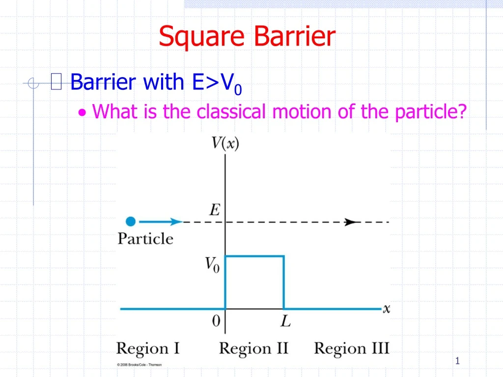
Square Barrier • Barrier with E>V0 • What is the classical motion of the particle?
Square Barrier • In regions I and III we need to solve • In region II we need to solve
Square Barrier • The solution in Region I contains the incident and reflected wave • The solution in Region III contains the transmitted wave • The solution in Region II is
Square Barrier • As usual we require continuity of ψ and dψ/dx at the boundaries • At x=0 this gives A and B in terms of C and D • At x=L this gives C and D in terms of E • The results are
Square Barrier • We define reflection R and transmission T coefficients • And I’ll leave it to you to show that R+T=1
Square Barrier • Using relations for k and kII, we can rewrite the transmission coefficient T as
Square Barrier • There is one interesting feature • With E and V0 fixed, the transmission coefficient T oscillates between 1 and a minimum value as the barrier width is varied • We call the wave in the case of T=1 a resonance • A resonance is obtained when kIIL=nπ • This means T=1 at values of L=λ/2 in region II • That is, a standing wave will exist in region II
Square Barrier • Barrier with E<V0 • What is the classical motion of the particle?
Square Barrier • In regions I and III we need to solve • In region II we need to solve
Square Barrier • The solution in Region I contains the incident and reflected wave • The solution in Region III contains the transmitted wave • The solution in Region II is
Square Barrier • We could again apply boundary conditions on ψ and dψ/dx • But it’s easier to note the difference between this case and the one previous is • Thus for E < V0, T becomes
Square Barrier • Thus we get a finite transmission probability T even though E < V0 • This is called tunneling • You can think of tunneling in terms of the uncertainty principle • As shown in Thornton and Rex, when the particle is in region II, the uncertainty in kinetic energy is V0 – E • The uncertainty in energy is comparable to the barrier height and there is a probability that particles could have sufficient energy to cross the barrier
Square Barrier • For κL >> 1, the tunneling probability T becomes • For rough estimates we can further approximate this as (see example 6.15 in Thornton and Rex) • The exponential shows the importance of the barrier width L over the barrier height V0
STM • Invented by Gerd Binnig and Heinrich Rohrer in 1982 • Nobel prize in 1986! • The basic idea makes use tunneling • When a sharp needle tip is placed less than 1 nm from a conducting material surface and a voltage applied between them, electrons can tunnel between the tip and surface • Since the tunnel current varies exponentially with the tip-surface distance, sub-nm changes in distance can be detected
STM • STM tip
STM • Tunneling through the potential barrier
STM • Raster scanning with constant Z • Raster scanning with constant tunneling current
STM • The STM tip is attached to piezoelectric elements (usually a tube) that precisely control the position in x-y-z • Used to control tip-surface distance (z) • Used to raster scan (x-y)
TIP STM • STM can also be used to manipulate atoms via van der Waals, tunneling, or electric field forces
Quantum Corrals • Electron in a corral of iron atoms on copper
Quantum Corrals • Electron in a corral of iron atoms
Alpha Decay • Geiger-Nuttall law • Nuclei with A > 150 are unstable with respect to alpha decay • An alpha particle (α) consists of a bound state of 2 protons and 2 neutrons (4He nucleus) • A(Z,N) → A(Z-2,N-2) + α • Effectively all of the energy released goes into the kinetic energy of the α
Alpha Decay • Geiger-Nuttall law • Radioactive half lives vary from ~10-6s to ~1017s but the alpha decay energies only vary from 4 to 9 MeV
Alpha Decay • Geiger-Nuttall law • The experimental data follow the Geiger-Nuttall law • A calculation of the quantum mechanic tunneling probability explained this law and was one of the early successes of quantum mechanics
Alpha Decay • Calculation of the decay probability W • Do this for 238U alpha decay with rN=7 F and Tα=4.2 MeV
Alpha Decay • Calculation of P and ν
Alpha Decay • Calculation of transmission probability T • Preliminaries • Calculate the height of the Coulomb barrier • Calculate the tunneling distance
Alpha Decay • The Coulomb barrier is not a square well • There is a way in quantum mechanics to calculate T correctly (called the WKB approximation) but for today we’ll just estimate the equivalent height and width of a square well • Use VC=20 MeV and r’=25 F
Alpha Decay • Calculation of T
Alpha Decay • Calculation of t1/2