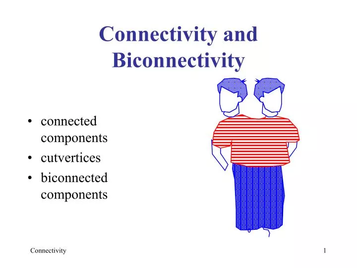
Connectivity and Biconnectivity

1. Connectivity and Biconnectivity • connected components • cutvertices • biconnected components

2. Connected Components • ConnectedGraph: any two vertices are connected by a path. • ConnectedComponent: maximal connected subgraph of a graph. connected component

3. Equivalence Relations • A relation on a set S is a set R of ordered pairs of elements of S defined by some property • Example: S = {1,2,3,4} R = {(i,j) S X S such that i < j} = {(1,2),(1,3),(1,4),(2,3),(2,4),{3,4)}

4. Equivalence Relations An equivalence relation is a relation with the following properties: (x,x) R,  x S (reflexive) (x,y) R (y,x) R (symmetric) (x,y), (y,z) R (x,z) R(transitive) The relation C can be defined as followson the set of vertices of a graph: (u,v) C u and v are in the same connected component C is an equivalence relation.

5. DFS on a Disconnected Graph • DFS(v) visits all the vertices and edges in the connected component of v. • To compute the connected components: k = 0 // component counter for each (vertex v) if unvisited(v) // add to component k the vertices //reached by v DFS(v, k++)

6. DFS on a Disconnected Graph A DFS from vertex a gives us...

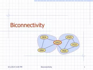
7. Cutvertices A Cutvertex (separation vertex) is one whose removal disconnects the graph. In the above graph, cutvertices are: ORD, DEN If the Chicago airport (ORD) is closed, then there is no way to get from Providence to cities on the west coast. Similarly for Denver.

8. BiconnectivityBiconnected graph: has no cutvertices • New flights: LGA-ATL and DFW-LAX make the graph biconnected.

9. Properties of Biconnected Graphs • There are two disjoint paths between any two vertices. • There is a cycle through any two vertices. By convention, two nodes connected by an edge form a biconnected graph, but this does not verify the above properties.

10. Biconnected Components • A biconnected component (block) is a maximal biconnected subgraph • Biconnected components are edge-disjoint but share cutvertices.

11. Characterization of the Biconnected Components We define an equivalence relationR on the edges of G: (e', e")R if there is a cycle containing both e' and e" How do we know this is an equivalence relation? Proof (by pretty picture) of the transitive property:

12. Characterization of the Biconnected Components • What does our equivalence relation R give us? • Each equivalence class corresponds to: • a biconnected component of G • a connected component of a graph H whose vertices are the edges of G and whose edges are the pairs in relation R.

13. DFS and Biconnected Components • Graph H has O(m2) edges in the worst case. • Instead of computing the entire graph H, we use a smaller proxy graph K. • The connected components of K are the same as those of H!

14. DFS and Biconnected Components • Start with an empty graph K whose vertices are the edges of G. • Given a DFS on G, consider the (m -n +1) cycles of G induced by the back edges. • For each such cycle C = (e0, e1, ... , ep) add edges (e0, e1) ... (e0, ep) to K.

15. A Linear Time Algorithm The size of K is O(mn) in the worst case. We can further reduce the size of the proxy graph to O(m) • Process the back edges according to a preorder visit of their destination vertex in the DFS tree • Mark the discovery edges forming the cycles • Stop adding edges to the proxy graph after the first marked edge is encountered. • The resulting proxy graph is a forest! • This algorithm runs in O(n+m) time.

16. Example • Back edges labeled according to the preorder visit of their destination vertex in the DFS tree Processing e1 Processing e2

17. Example (contd.) DFS tree final proxy graph (a tree since the graph is biconnected)

18. Why Preorder? The order in which the back edges are processed is essential for the correctness of the algorithm Using a different order ... ... yields a graph that provides incorrect information

19. Try the Algorithm on this Graph!