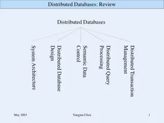
Distributed Databases

1. Distributed Databases CS347 Lecture 15 June 4, 2001

2. Topics for the day • Concurrency Control • Schedules and Serializability • Locking • Timestamp control • Reliability • Failure models • Two-phase commit protocol

3. Example constraint: X=Y X Y Node 1 Node 2 T1T2 1 a  X 5 c  X 2 X  a+100 6 X  2c 3 b  Y 7 d  Y 4 Y  b+100 8 Y  2d

4. Possible Schedule (node X) (node Y) 1 (T1) a  X 2 (T1) X  a+100 5 (T2) c  X 3 (T1) b  Y 6 (T2) X  2c 4 (T1) Y  b+100 7 (T2) d  Y 8 (T2) Y  2d If X=Y=0 initially, X=Y=200 at end Precedence: intra-transactioninter-transaction

5. Definition of a Schedule Let T= {T1, T2,…, TN} be a set of transactions. A schedule S over T is a partial order with ordering relation <S where: • S =  Ti • <S <i • for any two conflicting operations p,q S, either p <S q or q <S p Note: In centralized systems, we assumed S was a total order and so condition (3) was unnecessary.

6. Example (T1) r1[X]  w1[X] (T2) r2[X]  w2[Y]  w2[X] (T3) r3[X]  w3[X]  w3[Y]  w3[Z] r2[X]  w2[Y]  w2[X] S: r3[Y]  w3[X]  w3[Y]  w3[Z] r1[X]  w1[X]

7. Precedence Graph • Precedence graph P(S) for schedule S is a directed graph where • Nodes = {Ti | Tioccurs in S} • Edges = {Ti Tj |  p  Ti, q  Tj such that p, q conflict and p <S q} r3[X]  w3[X] P(S): T2 T1  T3 S: r1[X]  w1[X]  w1[Y] r2[X]  w2[Y]

8. Serializability Theorem: A schedule S is serializable iff P(S) is acyclic. Enforcing Serializability • Locking • Timestamp control

9. Distributed Locking • Each lock manager maintains locks for local database elements. • A transaction interacts with multiple lock managers. scheduler 1 scheduler N ….. locks for D1 locks for DN D1 DN node 1 access & lock data node N access & lock data T

10. Locking Rules • Well-formed/consistent transactions • Each transaction gets and releases locks appropriately • Legal schedulers • Schedulers enforce lock semantics • Two-phase locking • In every transaction, all lock requests precede all unlock requests. These rules guarantee serializable schedules

11. Locking replicated elements • Example: • Element X replicated as X1 and X2 on sites 1 and 2 • T obtains read lock on X1; U obtains write lock on X2 • Possible for X1 and X2 values to diverge • Possible that schedule may be unserializable • How do we get global lock on logical element X from local locks on one or more copies of X?

12. Primary-Copy Locking • For each element X, designate specific copy Xi as primary copy • Local-lock(Xi)  Global-lock(X) Synthesizing Global Locks • Element X with n copies X1 …. Xn • Choose “s” and “x” such that • 2x > n • s + x > n • Shared-lock(s copies)  Global-shared-lock(X) • Exclusive-lock(x copies)  Global-exclusive-lock(X)

13. Special cases Read-Lock-One; Write-Locks-All (s = 1, x = n) • Global shared locks inexpensive • Global exclusive locks very expensive • Useful when most transactions are read-only Majority Locking (s = x = (n+1)/2) • Many messages for both kinds of locks • Acceptable for broadcast environments • Partial operation under disconnected network possible

14. Supply proof. Theorem: If S is a schedule that satisfies TO rule, P(S) is acyclic (hence S is serializable). Timestamp Ordering Schedulers Basic idea: Assign timestamp ts(T) to transaction T. If ts(T1) < ts(T2) … < ts(Tn), then scheduler produces schedule equivalent to serial schedule T1 T2 T3 ….Tn. TO Rule: If pi[X] and qj[X] are conflicting operations, then pi[X] <S qj[X] iff ts(Ti) < ts(Tj).

15. ts(T1) < ts(T2) reject! abort T1 abort T1 abort T2 abort T2 Example (Node X) (Node Y) (T1) a  X (T2) d  Y (T1) X  a+100 (T2) Y  2d (T2) c  X (T1) b  Y (T2) X  2c (T1) Y  b+100

16. Strict T.O • Problem: Transaction reads “dirty data”. Causes cascading rollbacks. • Solution: Enforce “strict” schedules in addition to T.O rule Lock written items until it is certain that the writing transaction has committed. Use a commit bit C(X) for each element X. C(X) = 1 iff last transaction that last wrote X committed. If C(X) = 0, delay reads of X until C(X) becomes 1.

17. abort T1 (T2) c  X (T2) X  2c Revisit example under strict T.O ts(T1) < ts(T2) (Node X) (Node Y) (T1) a  X (T2) d  Y (T1) X  a+100 (T2) Y  2d (T2) c  X (T1) b  Y reject! delay abort T1

18. Enforcing T.O For each element X: MAX_R[X]  maximum timestamp of a transaction that read X MAX_W[X]  maximum timestamp of a transaction that wrote X rL[X]  number of transactions currently reading X (0,1,2,…) wL[X]  number of transactions currently writing X (0 or 1) queue[X]  queue of transactions waiting on X

19. T.O. Scheduler ri [X] arrives: • If (ts(Ti) < MAX_W[X]) abort Ti • If (ts(Ti) > MAX_R[X]) then MAX_R[X] = ts(Ti) • If (queue[X] is empty and wL[X] = 0) • rL[X] = rL[X]+1 • begin ri[X] • Else add (r,Ti) to queue[X] Note: If a transaction is aborted, it must be restarted with a larger timestamp. Starvation is possible.

20. T.O. Scheduler wi[X] arrives: • If (ts(Ti) < MAX_W[X] or ts(Ti) < MAX_R[X]) abort Ti • MAX_W[X] = ts(Ti) • If (queue[X] is empty and wL[X]=0 AND rL[X]=0) • wL[X] = 1 • begin wi[X] • wait for Ti to complete • Else add (w, Ti) to queue Work out the steps to be executed when ri[X] or wi[X] completes.

21. Thomas Write Rule MAX_R[X] MAX_W[X] ts(Ti) Ti wants to write X • wi[X] arrives: • If (ts(Ti) < MAX_R[X]) abort Ti • If (ts(Ti) < MAX_W[X]) ignore this write. • Rest as before…..

22. Optimization • Update MAX_R and MAX_W when operation is executed, not when enqueued. Example: • Multi-version timestamps W, ts=9 MAX_W[X] = 7 instead of 9 queue[X] W, ts=8 W, ts=7 active write ri[x] ts(Ti)=8 X: Value written with ts=9 Value written with ts=7 . . .

23. Think of examples for these cases. T1: w1[Y] T2: r2[X] r2[Y] w2[Z] ts(T1)<ts(T2)<ts(T3) T3: w3[X] Schedule S: r2[X] w3[X] w1[Y] r2[Y] w2[Z] 2PL  T.O T.O. schedules 2PL schedules

24. MAX_R MAX_W X1 X2 . . . . . . . . . . Xn Timestamp management • Too much space • Additional IOs

25. Timestamp Cache Item MAX_R MAX_W • If a transaction reads or writes X, make entry in cache for X (add row if required). • Choose tsMIN current time – d • Periodically purge all items X with MAX_R[X] < tsMIN & MAX_W[X] < tsMIN and store tsMIN. • If X has cache entry, use those MAX_R and MAX_W values. Otherwise assume MAX_R[X] = MAX_W[X] = tsMIN . X tsMIN Y . . . Z

26. Distributed T.O Scheduler scheduler 1 scheduler N ….. D1 ts cache DN ts cache D1 DN node 1 node 2 T • Each scheduler is “independent” • At end of transaction, signal all schedulers involved, • indicating commit/abort of transaction.

27. Reliability • Correctness • Serializability • Atomicity • Persistence • Availability

28. Types of failures • Processor failures • Halt, delay, restart, berserk, ... • Storage failures • Transient errors, spontaneous failures, persistent write errors • Network failures • Lost messages, out-of-order messages, partitions • Other ways of characterizing failures • Malevolent/Unintentional failures • Single/Multiple failures • Detectable/Undetectable failures

29. Models for Node Failure (1) Fail-stop nodes perfect halted recovery perfect Volatile memory lost Stable storage ok (2) Byzantine nodes perfect arbitrary failure recovery perfect At any given time, at most some fraction f of nodes have failed (typically f < 1/2 or f < 1/3)

30. Models for Network Failure (1) Reliable network • in order messages • no spontaneous messages • timeout TD Destination down If no ack in TD sec. • (2) Persistent messages • if destination is down, network will eventually deliver messages. • simplifies node recovery but inefficient (hides too much in network layer)

31. Models for Network Failure • (3) Partitionable network • in order messages • no spontaneous messages • no timeouts

32. Scenarios • Reliable network and Fail-stop nodes • No data replication (1) • Data replication (2) • Partitionable network and Fail-stop nodes • No data replication (3) • Data replication (4)

33. Scenario 1 Reliable network, fail-stop nodes, no data replication N net Item X • Key consequence: node N “controls” X • N is responsible for concurrency control and • recovery of X • Single control point for each data element • If N is down, X is unavailable

34. commit commit abort Distributed commit problem . Transaction T Action: a1,a2 Action: a3 Action: a4,a5

35. Distributed Commit • Make global decision on committing or aborting a distributed transaction • Assume atomicity mechanisms at each site ensure each local component is atomic • Each component either commits or has no effect on local database • Enforce rule that either all components commit or all abort

36. Centralized two-phase commit Coordinator State Transition Diagram Participant I I exec nok go exec* nok abort* exec ok W A W A ok* commit abort - commit - C C Notation: Incoming Message (* = everyone) Outgoing Message

37. Key Points • When participant enters “W” state: • It must have acquired all resources (e.g. locks) required for commit • But, it can only commit when so instructed by the coordinator • After sending “nok” participant can unilaterally abort. • Coordinator enters “C” state only if all participants are in “W”, i.e., it is certain that all participants will eventually commit.

38. Handling node failures • Coordinator and participant logs used to reconstruct state before failure. • Important that each message is logged before being sent • Coordinator failure may require leader election • Participant failure: recovery procedure depends on last log record for T • “C” record: commit T • “A” record: abort T • “W” record: obtain write locks for T and wait/ask coordinator or other participant • No log records for T: abort T

39. Example Participant log crash T1; X undo/redo info T1; Y undo/redo info T1 “W” state ... ... • During recovery at participant: • Obtain write locks for X and Y (no read locks) • Wait for message from coordinator • (or ask coordinator)

40. T1 start part={a,b} T1 OK from a RCV ... ... ... Logging at the coordinator Example: tracking who has sent “OK” msgs Log at coord: • After failure, we know still waiting for OK from node b • Alternative: do not log receipts of “OK”s. Simply abort T1

41. ping abort ping - _t_ cping _t_ abort* ping commit _t_ cping Coordinator (with timeouts and finish state) I nok abort* _go_ exec* W A ok* commit* nok* - C F c-ok* - t=timeout

42. cping done cping , _t - ping equivalent to finish state cping done “done” message counts as either c-ok or nok for coordinator Participant (with timeouts and finish state) exec nok I exec ok abort nok W A commit c-ok C

43. Presumed abort protocol • “F” and “A” states combined in coordinator • Saves persistent space (forget about a transaction quicker) • Presumed commit is analogous

44. Presumed abort-coordinator (participant unchanged) I ping abort nok, t abort* _go_ exec* ping - A/F W ok* commit* c-ok* - C ping commit _t_ cping

45. 2PC is blocking P4 Coordinator P1 P2 P3 W W W • Case I: P1  “W”; coordinator sent commits • P1  “C” • Case II: P1  NOK; P1  A • P2, P3, P4 (surviving participants) cannot safely abort or commit transaction

46. Variants of 2PC ok ok ok Linear Coordinator commit commit commit Hierarchical

47. Variants of 2PC Distributed • Nodes broadcast all messages • Every node knows when to commit

48. Resources • “Concurrency Control and Recovery” by Bernstein, Hardzilacos, and Goodman • Available at http://research.microsoft.com/pubs/ccontrol/ • Timestamp control • Chapter 9 of the CS245 Textbook (“Database System Implementation” by Garcia-Molina, Ullman, and Widom)