Download
1 / 28
280 likes | 294 Views
Lesson 3: Choosing from distributions. Choosing from distributions Discrete (Review) Continuous: Direct (Review) Continuous: Rejection Probability mixing Metropolis method Stratified sampling. Overview of pdf and cdf (Review). Basic definition of probability density function ( p.d.f .):

E N D
Lesson 3: Choosing from distributions • Choosing from distributions • Discrete (Review) • Continuous: Direct (Review) • Continuous: Rejection • Probability mixing • Metropolis method • Stratified sampling
Overview of pdf and cdf (Review) • Basic definition of probability density function (p.d.f.): • And its integral, the cumulative distribution function (c.d.f.):
Overview of pdf and cdf (2) • Corollaries of these definitions:
Mapping x->x using p(x) • Our basic technique is to use a unique y->x • y=x from (0,1) and x from (a,b) • We are going to use the mapping backwards
Mapping (2) Note that: • x(a)=0 • x(b)=1 • Function is non-decreasing over domain (a,b) Our problem reduces to: • Finding x(x) • Inverting to get x(x), a formula for turning pseudo-random numbers into numbers distributed according to desired p(x)
Mapping (3) • We must have:
Resulting general procedure • Form CDF: • Set equal to pseudo-random number: • Invert to get formula that translates from x to x:
Uniform distribution • For our first distribution, pick x uniformly in range (a,b): • Step 1: Form CDF.
Uniform distribution (2) • Step 2: Set pseudo-random number to CDF: • Step 3: Invert to get x(x): • Example: Choose m uniformly in (-1,1):
Discrete distribution • For a discrete distribution, we have N choices of state i, each with probability , so: • Step 1: Form CDF:
Discrete distribution (2) • Step 2: Set pseudo-random number to CDF: • Step 3: Invert to get x(x):
Discrete distribution (3) • Example: Choose among 3 states with relative probabilities of 4, 5, and 6.
Continuous distribution: Direct • This fits the “pure” form developed before. • Form CDF: • Set equal to pseudo-random number: • Invert to get formula that translates from x to x:
Continuous: Direct (2) • Example: Pick x from:
Testing your selection • There are two simple ways to check a routine that is used to choose from a given distribution: binning or moments • Binning involves dividing the domain (or part of it) into (usually equal-sized) regions and then counting what fraction of chosen values fall in the region. • The expected answer for a bin that goes from a to b is • This will be approximately equal to (and close enough for our purposes) the midpoint value times the width: • The text notes (and Public area) have a Java routine that will perform a bin testing • Hint: Do NOT code this with a IF test for each bin. Instead use the integer value of (chosen value)/(total width)*(number of bins)+1 to identify the bin that x goes into.
Continuous: Rejection • Basis of rejection approach: Usual procedure (using a flat x distribution): • Find a value • Choose • Keep iff Otherwise, return to 1.
Continuous: Rejection (3) • Example: Use rejection to pick x from:
Basic idea of probability mixing • Situations arise in which you have multiple distributions involved in a single decision:
Probability mixing procedure • Real problems do not present themselves so cleanly and you have to figure it out:
Probability mixing procedure (2) Procedure: • Form and normalize the • Choose the distribution i using these
Probability mixing procedure (3) Procedure: • Form the p.d.f. for distribution i: • Choose using
Probability mixing procedure (3) Example:Use probability mixing to select x from:
Metropolis • This is a very non-intuitive procedure that falls under the category of Markov Chain MC • It will ULTIMATELY deliver a consistent series of x’s distributed according to a desired functional form (which does NOT have to be normalized nor do you need to know a maximum value) • It has many advantages for certain physical problems in which the relative probability of a chosen point can be determined even if a closed form of the PDF is not available • The main disadvantage is that it is very hard to tell when the procedure has “settled in” to the point that the stream of x’s can be trusted to deliver a consistent distribution • This method was (supposedly) worked out as part of an after-dinner conversation in Los Alamos after WWII
Metropolis (2) • In its simplest form, the procedure is: • Choose x according to a distribution that has certain properties. We will not go into the details except to say that a uniform distribution has all the properties. • Evaluate the PDF at the chosen x • Decide whether to use the new point according to these rules: • IF the PDF evaluates higher than the PREVIOUSLY chosen point’s PDF, then use the new x • IF the PDF evaluates less than the previous point’s PDF, then pull another random number between 0 and 1 • If the new random number is LESS than the ratio of (new point’s PDF)/(old point’s PDF), then use the new x • If the previous test fails, then REUSE the old x
“Other”: Two alternate • Choose x from using: • Choose x from (Gaussian/normal) using: (Why 12?)