Download
1 / 15
150 likes | 333 Views
L1a to L2 Aquarius Processor Frank Wentz and Thomas Meissner. Aquarius Algorithm Workshop, Santa Rosa, CA, March 9-11, 2010. Signals Receive by Aquarius. Sun. Galaxy & Cosmic. Aquarius. Moon. Ionosphere. Atmosphere. Solar Backscatter. Quasi Specular. Solar Reflection. Land.

E N D
L1a to L2 Aquarius Processor Frank Wentz and Thomas Meissner Aquarius Algorithm Workshop, Santa Rosa, CA, March 9-11, 2010
Signals Receive by Aquarius Sun Galaxy & Cosmic Aquarius Moon Ionosphere Atmosphere Solar Backscatter Quasi Specular Solar Reflection Land Ocean Surface
L1a to L2 Aquarius Processor Subroutines that are called: call initialize call read_l1a call geolocation call count_to_TA call get_ancillary_data call fd_tb_toa call fd_tbsur_sss call fd_ta_expected call write_l2_arrays Green Boxes show L2 Outputs
Subroutine Initialize Floor value for galaxy radiation, treated like uniform cosmic background, subtract out of galaxy tables real(4), parameter :: tb_cos=3.0 Apply these to get effective eia real(8), parameter :: tht_coef(n_rad)=(/1.0017714d0, 1.0018588d0, 1.0014806d0/) Coefs for directional variable of surface emission. Currently set to 0 real(4), parameter :: dir_coef(4,2)=(/0.,0.,0.,0.,0.,0.,0.,0./) refl=refl - wind*((dir_coef(1,:)+dir_coef(2,:)*tht)*cosd(phir) - (dir_coef(3,:)+dir_coef(4,:)*tht)*cosd(2*phir)) Coefs for sun backscatter, currently set to 0 real(4), parameter :: bk_coef(3,2,n_rad)=(/0.,0.,0.,0.,0.,0.,0.,0.,0.,0.,0.,0.,0.,0.,0.,0.,0.,0./) tb_backscatter=bk_coef(1,:,irad)*flux*wind*(bk_coef(2,:,irad)*abs(celtht-suntht) + bk_coef(3,:,irad)*abs(celphi-sunphi)) Calibration constants for counts-to-ta process Discussed later this morning
Subroutine Initialize (cont) APC matrices real(4) apc_matrix(3,3,n_rad), apc_matrix_inv(3,3,n_rad) do istokes=1,3 tbtoi(istokes)=dot_product(apc_matrix(:,istokes,irad),taearth) enddo SSS Regression Algorithm real(4) sss_coef(4,251,451) sss_coef1=a1*b1*sss_coef(1,i1,j1) + a1*b2*sss_coef(1,i1,j2) + a2*b1*sss_coef(1,i2,j1) + a2*b2*sss_coef(1,i2,j2) sss_coef2=a1*b1*sss_coef(2,i1,j1) + a1*b2*sss_coef(2,i1,j2) + a2*b1*sss_coef(2,i2,j1) + a2*b2*sss_coef(2,i2,j2) sss_coef3=a1*b1*sss_coef(3,i1,j1) + a1*b2*sss_coef(3,i1,j2) + a2*b1*sss_coef(3,i2,j1) + a2*b2*sss_coef(3,i2,j2) sss_coef4=a1*b1*sss_coef(4,i1,j1) + a1*b2*sss_coef(4,i1,j2) + a2*b1*sss_coef(4,i2,j1) + a2*b2*sss_coef(4,i2,j2) sss=sss_coef1 + sss_coef2*surtb(1) + sss_coef3*surtb(2) + sss_coef4*win Meissner-Wentz Specular Reflectivity Coef: EIA,SST,SSS integer(2) ireflecv(901,371,226),ireflech(901,371,226) Direct and Reflected TA Sun and Galaxy Tables: (nomega=1441, nzang=1441, 0.25 deg) real(4) tasun_dir_tab(nomega,nzang,3,n_rad), tasun_ref_tab(nomega,nzang,3,n_rad) real(4) tagal_dir_tab(nomega,nzang,3,n_rad), tagal_ref_tab(nomega,nzang,3,n_rad,5) Fractional Land Tables: Within 3dB footprint and average over entire Earth, nlon_lnd=2160, nzang_lnd=2881 real(4) fpt_lnd(nlon_lnd,nzang_lnd,n_rad), frc_lnd(nlon_lnd,nzang_lnd,n_rad) Approximate Gain Pattern for Finding Sea Ice Contamination real(4) gain_ice(0:150,n_rad) Monthly Climatology SSS Table: Used for Computing Reflected Galaxy TA and Expected TA real(4) sss_tab(360,180,12) Monthly Climatology Surface Reflectivity Tables: Used for Computing Reflected Galaxy TA and Expected TA real(4) reflv_land_tab(360,181,12,3),reflh_land_tab(360,181,12,3)
Subroutine Read_L1A Simply reads in all the L1A variables and arrays for a single orbit. integer(4), parameter :: max_cyc= 5000 ! max number of block in l1a file = (5872 sec/orbit)*(1.2 overlap)/(1.44 sec/block) + slop integer(4), parameter :: n_rad=3 ! number of radiometers (i.e., horns) (inner, middle, outer) integer(4), parameter :: n_prt=85 ! number of thermistors integer(4), parameter :: n_subcyc=12 ! number of sub cycles per cycle integer(4), parameter :: npol=4 !number of polarizations (v, h, plus, minus) integer(4), parameter :: n_Sacc=6 ! number of S(short) accum (antenna) integer(4), parameter :: n_Lacc=8 ! number of L(long) accum (calibration) integer(4) iorbit, n_cyc real(8), dimension (max_cyc) :: time_utc_2000, time_ut1_2000 real(8), dimension(3,max_cyc) :: scpos_j2k, scvel_j2k, scrpy integer(4), dimension (max_cyc) :: iflag_qc real(4), dimension(n_prt,max_cyc) :: t_prt ! Short accummulation radiometer raw counts ! 6 records for each of the 12 subcycles. ! S1 and S2 are double accumulatons and will be divided by 2 during pocessing. ! Polarization order (last dimension) is 1=V, 2=P, 3=M, 4=H real(4), dimension(n_Sacc, n_subcyc, npol, n_rad, max_cyc) :: S_acc_raw ! raw SA counts ! Long accumulation radiometer raw counts ! 8 records per cycle. ! L1-L4 are to be divided by 10. L5-L8 are to be divided by 2. The divisions will be performed during processing. real(4), dimension(n_Lacc, npol, n_rad, max_cyc) :: L_acc_raw ! raw LA counts
Subroutine geolocation integer(4), dimension( max_cyc) :: iflag_sun real(8), dimension( max_cyc) :: zang, sclat, sclon, scalt real(8), dimension(3, max_cyc) :: sund, sunr, moond real(8), dimension(3,n_rad,max_cyc) :: bore_sight real(4), dimension( n_rad,max_cyc) :: cellat, cellon, celtht, celphi, suntht, sunphi, sunglt, moonglt, glxlat, glxlon real(4), dimension(4,n_rad,max_cyc) :: cellat_corners, cellon_corners iflag_sun= 1 if sun is visible from spacecraft (usual case), otherwise it = 0 zang= intra-orbit angle. it is zero at the south pole, 90 deg at the equator ascending node, etc. sclat= geodetic latitude of the spacecraft earth nadir point (deg) sclon= east longitude of the spacecraft earth nadir point (deg) scalt= spacecraft altitude, nadir point to spacecraft (meters) sund= earth-to-sun unit vector in eci coordinates sunr= unit vector from spacecraft to sun reflection point on earth in eci coordinates moond= earth-to-moon unit vector in eci coordinates bore_sight= unit vector from the spacecraft to the center of the observation cell cellat= geodetic latitude (deg) cellon= east longitude (deg) celtht= boresight earth incidence angle (deg) celphi= boresight earth-projection relative to clockwise from north (deg), boresight points towards earth suntht= sun vector earth incidence angle (deg) sunphi= sun vector earth_projection relative to clockwise from north (deg), sun vector points away from earth sunglt= sun glint angle: angle between the specular reflected boresight vector and the sun vector (deg) mooonglt= moon glint angle: angle between the specular reflected boresight vector and the moon vector (deg) glxlat= j2k declination latitude from where the specular galactic radiation originated (deg) glxlon= j2k ascension from where the specular galactic radiation originated (deg) cellat_corners= geodetic latitudes of the four corners of the 3-db footprint cellon_corners = east longitudes of the four corners of the 3-db footprint Software for geolocation is based on standard methods with accuracy <= 100 meters
Subroutine count_to_ta This routine was written by Thomas Meissner in close coordination with Jeff Piepmeier It was verified by doing closure runs: count TA count Embedded in the routine is currently a placeholder for RFI detection. Chris Ruf recently delivered RFI detection code that we will implement in the coming weeks. Discussed later this morning
Subroutine get_ancillary_data real(4), dimension( max_cyc) :: solar_flux real(4), dimension(n_rad,max_cyc) :: fland, gland, fice, gice, sss_climate, surtep, winspd, windir, tran, tbup, tbdw solar_flux= solar flux (sfu) fland = fraction of land within 3db footprint (0 to 1.0) gland= fraction of land over entire gain pattern (0 to 1.0) fice= fraction of sea ice at boresight (0 to 1.0) gice= fraction of sea ice over entire gain pattern (0 to 1.0) sss_climate= salinity climatology (psu) surtep = ncep surface temp (kelvin) winspd = ncep wind speed (m/s) windir= ncep wind direction (deg) tran= one-way atmospheric transmission (0 to 1) tbup= upwelling atmospheric brightness temperature (k) tbdw= downwelling atmospheric brightness temperature (k) • Ancillary data comes from: • 1. Simulator: land fraction • NCEP: sea ice, surface temperature, wind speed and direction, tran, tbup, tbdw • TBD: solar flux and salinity climatology • 3-D Interpolation of tables in latitude, longitude, and time used to get value at Aquarius footprint
Subroutine fd_tb_toa real(4), dimension(3,n_rad,max_cyc) :: tagal_dir, tagal_ref, t asun_dir, tasun_ref, ta_earth tagal_dir= direct galaxy radiation in terms of classical stokes (K) tagal_ref = reflected galaxy radiation in terms of classical stokes (K) tasun_dir= direct solar radiation in terms of classical stokes (K) tasun_ref= reflected solar radiation in terms of classical stokes (K) ta_earth= TA just from earth with galaxy and sun removed in term of vpol, hpol, 3rd stokes (K) Arrays tagal_dir, tagal_ref, tasun_dir, and tasun_ref are computed from tables generated by the simulator given the satellite position and time of year and ascending node local time. Subtract direct and reflected sun radiation (optional) and subtract direct galaxy from TA measurement: ta_earth=tamea - tagal_dir- iopt(1)*tasun_dir - iopt(2)*tasun_ref Adjust table value of reflected galaxy radiation to correspond to actual surface reflectivity and atmos. transmittance Then subtract the adjusted value from the TA measurement: call adjust_tagal_ref(irad,refl0,refl,transq0,transq,taearth,tagal_ref, tagal_ref_adj) tagal_ref=tagal_ref_adj ta_earth=ta_earth - tagal_ref
Subroutine fd_tb_toa (cont.) real(4), dimension(3,n_rad,max_cyc) :: tb_toi real(4), dimension(2,n_rad,max_cyc) :: tb_toa real(4), dimension( n_rad,max_cyc) :: faraday_deg tb_toi= top of ionosphere brightness temperature in term of vpol, hpol, 3rd stokes (K) tb_toa = top of atmosphere brightness temperature in term of vpol, hpol faraday_deg= faraday rotation angle (deg) APC correction to convert TA to TOI TB: do istokes=1,3 tb_toi(istokes)=dot_product(apc_matrix(:,istokes,irad),ta_earth) enddo Compute Faraday rotation: faraday_deg(irad,icyc)=0.5*atand(tb_toi(3)/tb_toi(2)) Remove Faraday rotation to convert TOI TB to TOA TB: tb_toa(1)=tb_toi(1) tb_toa(2)=sqrt(tb_toi(2)**2 + tb_toi(3)**2) Store TA and TB values as modified Stokes: call stokes_to_vh( ta_earth) call stokes_to_vh( tb_toi) call stokes_to_vh( tb_toa)
Subroutine fd_tbsur_sss real(4), dimension(2,n_rad,max_cyc) :: tb_sur real(4), dimension( n_rad,max_cyc) :: sss_aquarius tb_sur = surface brightness temperature, ie emissivity times temperature, in term of vpol, hpol sss_aquarius = aquarius salinity retrieval (psu) do icyc=1,n_cyc do irad=1,n_rad thtadj=tht_coef(irad)*celtht(irad,icyc) !apply a very small adjustment to incidence angle to get effective incidence angle phir=celphi(irad,icyc) - windir(irad,icyc) !relative azimuth angle, 0=upwind sst=surtep(irad,icyc) - 273.15 tbdown=tbdw(irad,icyc)+ tran(irad,icyc)*tb_cos !tb_cos = 3 K call fd_sun_backscatter(irad,solar_flux(icyc),thtadj,celphi(irad,icyc),suntht(irad,icyc),sunphi(irad,icyc),winspd(irad,icyc), tb_backscatter) surtb=(tb_toa( :,irad,icyc) - tbup(irad,icyc))/tran(irad,icyc) - tb_backscatter emiss=(surtb - tbdown)/(surtep(irad,icyc) -tbdown) surf_emission=emiss*surtep(irad,icyc) tb_sur( :,irad,icyc)=surf_emission ! remove direction component of surface emssion to get isotropic surface emission surf_emission0=surf_emission - winspd(irad,icyc)*((dir_coef(1,:)+dir_coef(2,:)*thtadj)*cosd(phir) – (dir_coef(3,:)+dir_coef(4,:)*thtadj)*cosd(2*phir)) ! estimate sea-surface salinity if(sst.lt.-5.000) sst=-5.000 if(sst.gt.39.999) sst=39.999 call fd_sss(thtadj,sst,winspd(irad,icyc),surf_emission0, sss_aquarius(irad,icyc)) enddo !irad enddo !icyc
Subroutine fd_ta_expected real(4), dimension(3,n_rad,max_cyc) :: ta_expected ta_expected = expected ta measurement computed from all the ancillary data in term of vpol, hpol, 3rd stokes (K) call find_refl_tot(irad,idayjl,isecdy,cellat(irad,icyc),cellon(irad,icyc),thtadj,phir, fland(irad,icyc),fice(irad,icyc),sss_climate(irad,icyc),sst,winspd(irad,icyc), refl) emiss=1 - refl tbdown=tbdw(irad,icyc)+ tran(irad,icyc)*tb_cos call fd_sun_backscatter(irad,solar_flux(icyc),thtadj,celphi(irad,icyc),suntht(irad,icyc),sunphi(irad,icyc),winspd(irad,icyc), tb_backscatter) tbtoa=tbup(irad,icyc) + tran(irad,icyc)*(emiss*surtep(irad,icyc) + (1-emiss)*tbdown + tb_backscatter) call vh_to_stokes( tbtoa) tbtoi(1)=tbtoa(1) tbtoi(2)=tbtoa(2)*cosd(2*faraday_deg(irad,icyc)) tbtoi(3)=tbtoa(2)*sind(2*faraday_deg(irad,icyc)) do istokes=1,3 taexpected(istokes)=dot_product(apc_matrix_inv(:,istokes,irad),tbtoi) enddo taexpected=taexpected + tagal_dir(:,irad,icyc) + tagal_ref(:,irad,icyc) + iopt(1)*tasun_dir(:,irad,icyc) + iopt(2)*tasun_ref(:,irad,icyc) call stokes_to_vh( taexpected) ta_expected(:,irad,icyc)=taexpected
Subroutine fd_sss Train estimator to minimize (in a least-squares sense) the difference between the estimate of salinity given by the following expression and the true salinity. Appropriate noise is added to both the Tb values and the wind value when doing the training. ! Interpolate pre-computed sss_coef to actual incidence angle and sst brief=10*(tht-25.) i1=int(1+brief) i2=i1+1 a1=i1-brief a2=1.-a1 brief=10*(sst+5.) j1=int(1+brief) j2=j1+1 b1=j1-brief b2=1.-b1 sss_coef1=a1*b1*sss_coef(1,i1,j1)+ a1*b2*sss_coef(1,i1,j2) + a2*b1*sss_coef(1,i2,j1) + a2*b2*sss_coef(1,i2,j2) sss_coef2=a1*b1*sss_coef(2,i1,j1)+ a1*b2*sss_coef(2,i1,j2) + a2*b1*sss_coef(2,i2,j1) + a2*b2*sss_coef(2,i2,j2) sss_coef3=a1*b1*sss_coef(3,i1,j1)+ a1*b2*sss_coef(3,i1,j2) + a2*b1*sss_coef(3,i2,j1) + a2*b2*sss_coef(3,i2,j2) sss_coef4=a1*b1*sss_coef(4,i1,j1)+ a1*b2*sss_coef(4,i1,j2) + a2*b1*sss_coef(4,i2,j1) + a2*b2*sss_coef(4,i2,j2) ! Compute estimate of salinity sss=sss_coef1 + sss_coef2*surtb(1) + sss_coef3*surtb(2) + sss_coef4*win
Work To Be Done • Continue to Analysis 2007 Simulation Results to better Understand the Problem we are facing • Implement ancillary data routines for obtaining Solar Flux and “real-time” salinity. • Upgrade simulator to process data on a daily basis and send to ADF. • Generate TA Galaxy Reflection Tables for Rough Ocean Surfaces • Generate Land Correction Tables • Implement flags into the L2 data. • Implement moon in antenna main lobe • And, all the things I have forgotten