Download
1 / 53
590 likes | 724 Views
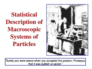
Delve into the fundamental concepts of statistical mechanics as applied to systems of particles. This chapter introduces the abstract ideas and concepts in Chs. 2 & 3, outlining the essential ingredients for a statistical description of systems with many particles. Explore the system state, choose a statistical ensemble, formulate basic postulates on probabilities, and conduct probability calculations. Understand the difference between macrostates and microstates, and the quantum and classical descriptions of systems. Learn how to predict probabilities using statistical methods and the importance of a priori probabilities in describing physical systems.

E N D
Preliminary Comments • Chs. 2 & 3 are, in many places, very abstract! • Difficulties students have with this material are often because of
Preliminary Comments • Chs. 2 & 3 are, in many places, very abstract! • Difficulties students have with this material are often because of the abstract ideas & concepts. • On the other hand, the math in these chapters is relatively straightforward. • I assure you that the material will become less abstractas we proceed through the course.
Discussion of the General Problem • We’ve reviewed elementary probability & statistics. • Now, we are finally ready to talk about PHYSICS • In this chapter (& the rest of the course) we’ll combine statistical ideas with the Laws of ClassicalorQuantum Mechanics≡ Statistical Mechanics
Discussion of the General Problem Laws of ClassicalorQuantum Mechanics≡ Statistical Mechanics • We can use either a classical or a quantum description of a system. • Of course, which is valid obviously depends on the problem!!
Four Essential Ingredientsfor a Statistical Description of a Systemwith many particles: (~ outline of Ch. 2!) 1. Specify “the System State”.
Four Essential Ingredientsfor a Statistical Description of a Systemwith many particles: (~ outline of Ch. 2!) 1. Specify “the System State”. 2. Choose a Statistical Ensemble
Four Essential Ingredientsfor a Statistical Description of a Systemwith many particles: (~ outline of Ch. 2!) 1. Specify “the System State”. 2. Choose a Statistical Ensemble 3. Formulate a Basic Postulate aboutà-prioriProbabilities.
Four Essential Ingredientsfor a Statistical Description of a Systemwith many particles: (~ outline of Ch. 2!) 1. Specify “the System State”. 2. Choose a Statistical Ensemble 3. Formulate a Basic Postulate aboutà-prioriProbabilities. 4. Do Probability Calculations
Four Essential Ingredientsfor a Statistical Description of a System with many particles: (~ outline of Ch. 2!) 1. Specify “the System State”. The state referred to here is the “System Macrostate”. • We’ll thoroughly discuss what we mean by “Macrostate” & we’ll also discuss that this is very different than the “Microstate of the System”! • We’ll also need a detailed method for specifying the Macrostate. This is discussed in this chapter.
Specification of the System State Microstate Microscopic System State • Quantum Description of the System: This means specifying a (large!) set of quantum numbers. • Classical Description of the System: This means specifying a point in a large dimensional phase space.
Macrostate Macroscopic System State • Quantum Description of the System: • For an isolated system, this means specifying a subset of the quantum states of the system. • The system is described by macroscopic parameters (that can be measured).
2. Statistical Ensemble: • We need to decide exactly which ensemble to use. This is also discussed in this chapter. In either Classical Mechanics or Quantum Mechanics: • If we had a detailed knowledge of all positions & momenta of all system particles & if we knew all inter-particle forces, we could (in principle) set up & solve the coupled, non-linear differential equations of motion, we could find EXACTLY the behavior of all particles for all time!
If we could set up & solve the coupled, non-linear differential equations of motion, we could (in principle) find EXACTLY the behavior of all particles for all time! • In practice we don’t have enough information to do this. Even if we did, such a problem is Impractical, if not Impossible to solve! • Instead, we’ll use Statistical/Probabilistic Methods.
Statistical/Probabilistic Methods: Require choosing an Ensemble • Lets think of doing MANY (≡ N) similar experiments on the system of particles we are considering. In general, the outcome of each experiment will be different. • So, we ask for the PROBABILITY of a particular outcome. This PROBABILITY≡ the fraction of cases out of N experiments which have that outcome. • This is how probability is determined by experiment. A goal of STATISTICAL MECHANICS is to predict this probability theoretically.
Next, we need to start somewhere, so we need to assume 3. A Basic Postulateabout à-prioriProbabilities. • “à-priori” ≡ prior(based on all of our prior knowledge of the system). • Our knowledge of a given physical system leads is to expect that there is NOTHING in the laws of mechanics (classical or quantum) which would result in the system preferring to be in any particular one of it’s Accessible (micro) States.
Webster’s on-line Dictionary: Definition of“à-priori” 1a:Deductive 1b:Relating to or derived by reasoning from self-evident propositions. a synonymto“à-posteriori” 1c: Presupposed by experience. 2a: Being without examination or analysis. analysis :Presumptive 2b: Formed or conceived beforehand
3. Basic Postulate about à-priori Probabilities. • There is NOTHING in the laws of mechanics (classical or quantum) which would result in the system preferring to be in any particular one of it’s Accessible Microstates.
3. Basic Postulate about à-priori Probabilities. • So, (if we have no contrary experimental evidence) we make the hypothesisthat: it is equally probable (or equally likely) that the system is inANY ONE of it’s accessible microstates.
The hypothesisis that it is equally probable (equally likely) that the system is in ANY ONEof it’s accessible microstates. • This postulate is reasonable & doesn’t contradict any laws of mechanics (classical or quantum). Is it correct? • That can only be confirmed by checking theoreticalpredictions & comparing those to experimental observation! Physics is an experimental science!! Often, this postulateis called The Fundamental Postulate of (Equilibrium) Statistical Mechanics!
4. Probability Calculations • Finally, we can do some calculations! • Once we have the Fundamental Postulate, we can use Probability Theory to predict the outcome of experiments. • Now, we will go through steps 1., 2., 3., 4. again in detail!
Statistical Formulation of the Mechanical Problem Section 2.1: Specification of the System State ≡Microstate • Consider any system of particles. We know that the particles will obey the laws of Quantum Mechanics (we’ll discuss theClassicaldescription shortly). • We’ll emphasize the Quantum treatment.
Consider any system of particles. • Using the Quantum treatment, consider a system with f degrees of freedom which can be described by a (many particle!) wavefunction Ψ(q1,q2,….qf,t), where q1,q2,….qf ≡ Set of f generalized coordinates required to characterize the system (needn’t be position coordinates!)
For a system with f degrees of freedom, the many particle wavefunction is formally: Ψ(q1,q2,….qf,t), q1,q2,….qf ≡ a set of f generalized coordinates which are required to characterize the system. • A particular quantum state (microstate) of the system is specified by giving values of some set of f quantum numbers. If we specify Ψat a given time t, we can (in principle) calculate it at any later time by solving the appropriate Schrödinger Equation
Now, lets look at some simple examples, which might also cause us to review some elementary Quantum Mechanics for you.
Example 1 • The system is a single particle, fixed in position. • It has intrinsic spin S = ½ &Intrinsic Angular Momentum = ½ћ. • In the Quantum Description of this system, the state of the particle is specified by specifying the projection m of this spin along a fixed axis (which we usually call the z-axis). • The quantum number m can thus have 2 values: ½ (“spin up”) or -½ (“spin down”) So, there are 2 possible microstates of the system.
Example 2 • The system is N particles (non-interacting), fixed in position. Each has intrinsic spin ½ soEACHparticle’s quantum number mi (i = 1,2,…N) can have one of the 2 values ½. Suppose that N is HUGE:N ~ 1024. • The microstate of this system is then specified by specifying the values of EACH of the quantum numbers: m1,m2, .. mN. There are(2)Nunique microstates of the system! WithN ~ 1024, this number isHUGE!!!
Example 3 • A system with N = 3 Particles, fixed in position, each with spin = ½ Each spin is either “up” (↑, m = ½) or “down” (↓, m = -½). • Each particle has a vector magnetic moment μ. • The projection of μalong a “z-axis” is either: μz = μ, for spin “up” or μz = -μ, for spin “down”
Put this system in an External Magnetic Field H. • Classical E&M tells us that a particle with magnetic moment μin an external field H has energy: ε = - μH • Combine this with the Quantum Mechanical result: • This tells us that each particle has 2 possible energies: ε+ ≡ - μHfor spin “up” ε- ≡ μHfor spin “down” So, for 3 particles, the Microstateof the system is specified by specifying each m = ½ There are(2)3 = 8 Possible Microstates!!
Possible States of a 3 Spin System • Given that we know no other information about • this system, all we can say about it is that • It has Equal Probabilityof Being Found • in Any Oneof These 8 States.
Example 4 • The system is a quantum mechanical, one-dimensional, simple harmonic oscillator, with position coordinate x & classical frequency ω. So the Quantum Energy of this system is: En = ћω(n + ½), (n = 0,1,2,3,….). • The quantum states of this oscillator are then specified by specifying the quantum number n. So, there are essentially an NUMBER of such states!
Example 5 • The system is N quantum mechanical, one-dimensional, simple harmonic oscillators, at positions xi, with classical frequencies ωi (i = 1,2,.. N). • The Quantum Energies of each particle in this system are: Ei = ћωi(ni + ½), (ni = 0,1,2,3,….). • The system’s quantum states are specified by specifying the values of eachquantum number ni. Here also, there are essentially an NUMBER of such states. • But, there are also a larger number of these than in Example 4!
Example 6 • The system is one particle, of mass m, confined to a rectangular box, but otherwise free. Taking the origin at a corner: 0 ≤ x ≤ Lx, 0 ≤ y ≤ Ly, 0 ≤ z ≤ Lz The particle is described by the QM wavefunction ψ(x,y,z), a solution to the Schrödinger Equation [-ћ2/(2m)][(∂2/∂x2) + (∂2/∂y2) + (∂2/∂z2)]ψ(x,y,z) = Eψ(x,y,z)
Wavefunction ψ(x,y,z), is a solution to [-ћ2/(2m)][(∂2/∂x2) + (∂2/∂y2) + (∂2/∂z2)]ψ(x,y,z) = Eψ(x,y,z) • Using the boundary condition that ψ = 0 on the box faces, it can be shown that: ψ(x,y,z) = [8/(LxLyLz)]½sin(nxπ/Lx)sin(nyπ/Ly)sin(nzπ/Lz) • nx, ny, nz are 3 quantum numbers (positive or negative integers).
ψ(x,y,z) = [8/(LxLyLz)]½sin(nxπ/Lx)sin(nyπ/Ly)sin(nzπ/Lz) • nx, ny, nz = 3 quantum numbers (positive or negative integers). • So, the particleQuantum Energy is: E = [(ћ2π2)/(2m)][(nx2/Lx2) + (ny2/Ly2) + (nz2/Lz2)] • The quantum states of this system are found by specifying the values of nx, ny, nz. • Again, there are essentially also an Number of such states.
Example 7 • N particles, non-interacting, of mass m, confined to a rectangular box. Take the origin at a corner 0 ≤ x ≤ Lx, 0 ≤ y ≤ Ly, 0 ≤ z ≤ Lz. • Since they are non-interacting, each particle is described by the QM wavefunction ψi(x,y,z), which is a solution to the Schrödinger Equation [-ћ2/(2m)][(∂2/∂x2) + (∂2/∂y2) + (∂2/∂z2)]ψi(x,y,z) = Eiψi(x,y,z)
N particles of mass m in a rectangular box. 0 ≤ x ≤ Lx, 0 ≤ y ≤ Ly, 0 ≤ z ≤ Lz. The QM wavefunction ψi(x,y,z), is a solution to [-ћ2/(2m)][(∂2/∂x2) + (∂2/∂y2) + (∂2/∂z2)]ψi(x,y,z) = Eiψi(x,y,z) • Using the boundary condition that ψ = 0 on the box faces: ψi(x,y,z) = [8/(LxLyLz)]½sin(nxπ/Lx)sin(nyπ/Ly)sin(nzπ/Lz) • nx, ny, nz are 3 quantum numbers (positive or negative integers).
ψ(x,y,z) = [8/(LxLyLz)]½sin(nxπ/Lx)sin(nyπ/Ly)sin(nzπ/Lz) • nx, ny, nz are 3 quantum numbers (positive or negative integers). • Each particle’sQuantum Energy is: E = [(ћ2π2)/(2m)][(nx2/Lx2) + (ny2/Ly2) + (nz2/Lz2) • The quantum states of this system are found by specifying the values of nx, ny, nz. for each particle. • Again, there are essentially also an Number of such states.
What about a Classical Descriptionof the Microstate of a many particle system? • Of course, the Quantum Description is always correct! • However, it is often useful & convenient to make the Classical Approximation. How do we specifythe Microstate of the system then?
Lets start with a very simple case: A Single Particle in 1 Dimension: • In classical mechanics, it can be completely described in terms of it’s generalized coordinate q & it’s momentum p. • The usual case is to consider the Hamiltonian Formulation of classical mechanics, where we talk of generalized coordinates q & generalized momenta p, rather than the Lagrangian Formulation, where we talk of coordinates q & velocities (dq/dt).
Of course, the particle obeys Newton’s 2nd Law under the action of the forces on it. Equivalently, it obeys Hamilton’s Equations of Motion. • q & p completely describe the particle classically. Given q, p at any initial time (say, t = 0), they can be determined at any other time t by integrating the equations of motion.
Given q, p at time t = 0, they can be determined at any other time t by integrating the Newton’s 2nd Law Equations of Motion forward in time. Knowing q & p at t = 0 in principle allows us to know them for all time t. q&pcompletely describethe particlefor all time. • This situation can be abstractly represented in a geometric way discussed on the next page.
At any time t, stating the (q, p) of the particle describes it’s • “Microstate” • Specification of the • “Particle Microstate” • is done by stating which point in this plane the particle “occupies”. • Consider the (abstract) 2-dimensional space defined by q, p:≡ “Classical Phase Space”of the particle. • Of course, as q & p change in time, according to • the equations of motion, the point representing the • particle “State”moves in the plane.
To do this, it is convenient to • subdivide the ranges of q & p • into very small rectangles of size: • qp. • q, p are continuous variables, so an number of points are in this 2-Dimensional Classical“Phase Space” • We want to describe the particle “Microstate”classically in a way that the number of states is countable. • Think of this 2-d phase space as divided into small cells of equal area: qp ≡ ho • ho ≡ a small (arbitrary) constant with units of angular momentum .
The 2-d phase space has a large number cells of area: qp = ho. • The (classical) particle “Microstate” is specified by stating which cell in phase space the q, p of the particle is in. Or, by stating that it’s coordinate lies between q & q + q & that it’s momentum lies between p & p + p. • “Microstate” • The phase space cell • labeled by the (q,p) that • the particle “occupies”.
This involves the “small” parameter ho, which is arbitrary. As a side note, however, we can use Quantum Mechanics & the Heisenberg Uncertainty Principle: “It is impossible toSIMULTANEOUSLY specify a particle’s position & momentum to a greater accuracy thanqp ≥ ½ћ” • So, the minimum value ofhois clearly ½ћ. As ho½ћ, the classical description of the Microstate approaches the quantum description & becomes more & more accurate.
Now!! Lets generalize all of this to a MANY PARTICLE SYSTEM • 1 particle in 1 dimension means we have to deal with a 2-dimensionalphase space. • The generalization to N particles is straightforward, but requires thinking in terms of a very abstract Multidimensionalphase space. • Consider a system with f degrees of freedom (f 1024): The system is described classically by f generalized coordinates:q1,q2,q3, …qf f generalized momenta:p1,p2,p3, …pf.
A complete description of the classical “Microstate” of the system requires the specification of: f generalized coordinates: q1,q2,q3, …qf. & f generalized momenta: p1,p2,p3, …pf (N particles, 3-dimensions f = 3N !!)
A complete description of the classical “Microstate” of the system requires the specification of: f generalized coordinates: q1,q2,q3, …qf. & f generalized momenta: p1,p2,p3, …pf (N particles, 3-dimensions f = 3N !!) • So, now lets think VERYabstractly in terms of a 2f-dimensional phase space
A complete description of the classical “Microstate” of the system requires the specification of: f generalized coordinates: q1,q2,q3, …qf. & f generalized momenta: p1,p2,p3, …pf (N particles, 3-dimensions f = 3N !!) • So, now lets think VERYabstractly in terms of a 2f-dimensional phase space • The system’s f generalized coordinates: q1,q2,q3, …qf. & f generalized momenta: p1,p2,p3, …pf are regarded as a point in the 2f-dimensional phase spaceof the system.