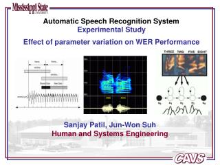
Automatic Speech Recognition (ASR): A Brief Overview

1. Automatic Speech Recognition (ASR): A Brief Overview

2. Radio Rex – 1920’s ASR

3. Statistical ASR • i_best = argmax P(M |X ) = argmax P(X|M ) P(M )(1st term, acoustic model; 2nd term,language model) • P(X|M )  P(X|Q ) [Viterbi approx.]where Qis the best state sequence in M • approximated by product of local likelihoods (Markov,conditional independence assumptions) i i i i i i M i i M i

4. Automatic Speech Recognition Speech Production/Collection Pre-processing Feature Extraction Hypothesis Generation Cost Estimator Decoding

5. Simplified Model of SpeechProduction Periodic Source Filters Random Source Vocal vibration or turbulence (Fine spectral structure) Vocal tract, nasal tract, radiation (spectral envelope)

6. Pre-processing Speech RoomAcoustics LinearFiltering Sampling & Digitization Microphone Issues: Noise and reverb, effect on modeling

7. Framewise Analysis of Speech Frame 1 Frame 2 Feature VectorX1 Feature VectorX2

8. Feature Extraction SpectralAnalysis AuditoryModel/ Orthogonalize (cepstrum) Issues: Design for discrimination, insensitivities to scaling and simple distortions

9. Representations are Important Network Speech waveform 23% frame correct Network PLP features 70% frame correct

10. Mel Frequency Scale

11. Spectral vs Temporal Processing Analysis (e.g., cepstral) frequency Spectral processing Time Processing (e.g., mean removal) frequency Temporal processing

12. a cat not is adog Hypothesis Generation cat dog a dog is not a cat Issue: models of language and task

13. Cost Estimation • Distances • -Log probabilities, from • discrete distributions • Gaussians, mixtures • neural networks

14. Nonlinear Time Normalization

15. Decoding

16. Pronunciation Models

17. Language Models • Most likely words for largest product • P(acousticswords)  P(words) • P(words) =  P(wordshistory) • bigram, history is previous word • trigram, history is previous 2 words • n-gram, history is previous n-1 words

18. Language Model RecognizedWords “zero” “three” “two” Cepstrum Probabilities“z” -0.81“th” = 0.15“t” = 0.03 Decoder Signal Processing Acoustic ProbabilityEstimator (HMM state likelihoods) ASR System Architecture Speech Signal Pronunciation Lexicon

19. HMMs for Speech • Math from Baum and others, 1966-1972 • Applied to speech by Baker in theoriginal CMU Dragon System (1974) • Developed by IBM (Baker, Jelinek, Bahl,Mercer,….) (1970-1993) • Extended by others in the mid-1980’s

20. Hidden Markov model (graphical form) q q q q 1 2 3 4 x x x x 1 2 3 4

21. Hidden Markov Model(state machine form) P(x | q ) P(x | q ) P(x | q ) 1 2 3 q q q 2 1 3 P(q | q ) P(q | q ) P(q | q ) 2 1 3 2 4 3

22. 1 2 1 2 1 1 1 2 1 2 2 Markov model q q 1 2 P(x ,x |q ,q )  P( q ) P(x |q ) P(q | q ) P(x | q )

23. HMM Training Steps • Initialize estimators and models • Estimate “hidden” variable probabilities • Choose estimator parameters to maximizemodel likelihoods • Assess and repeat steps as necessary • A special case of ExpectationMaximization (EM)

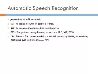
24. Progress in 3 Decades • From digits to 60,000 words • From single speakers to many • From isolated words to continuousspeech • From no products to many products,some systems actually saving LOTSof money

25. Real Uses • Telephone: phone company services(collect versus credit card) • Telephone: call centers for queryinformation (e.g., stock quotes, parcel tracking) • Dictation products: continuous recognition, speaker dependent/adaptive

26. But: • Still <97% on “yes” for telephone • Unexpected rate of speech causes doublingor tripling of error rate • Unexpected accent hurts badly • Performance on unrestricted speech at 70%(with good acoustics) • Don’t know when we know • Few advances in basic understanding

27. Why is ASR Hard? • Natural speech is continuous • Natural speech has disfluencies • Natural speech is variable over:global rate, local rate, pronunciationwithin speaker, pronunciation acrossspeakers, phonemes in differentcontexts

28. Why is ASR Hard?(continued) • Large vocabularies are confusable • Out of vocabulary words inevitable • Recorded speech is variable over:room acoustics, channel characteristics,background noise • Large training times are not practical • User expectations are for equal to orgreater than “human performance”

29. ASR Dimensions • Speaker dependent, independent • Isolated, continuous, keywords • Lexicon size and difficulty • Task constraints, perplexity • Adverse or easy conditions • Natural or read speech

30. Telephone Speech • Limited bandwidth (F vs S) • Large speaker variability • Large noise variability • Channel distortion • Different handset microphones • Mobile and handsfree acoustics

31. Hot Research Problems • Speech in noise • Multilingual conversational speech (EARS) • Portable (e.g., cellular) ASR • Question answering • Understanding meetings – or at least browsing them

32. Hot Research Approaches • New (multiple) features and models • New statistical dependencies • Multiple time scales • Multiple (larger) sound units • Dynamic/robust pronunciation models • Long-range language models • Incorporating prosody • Incorporating meaning • Non-speech modalities • Understanding confidence

33. Multi-frame analysis • Incorporate multiple frames as a single observation • LDA the most common approach • Neural networks • Bayesian networks (graphical models, including Buried Markov Models)

34. Linear Discriminant Analysis (LDA) All variables for several frames x 1 x 2 y 1 = X x y 3 2 x 4 Transformation to maximize ratio: between-class variance within-class variance x 5

35. Multi-layer perceptron

36. Buried Markov Models

37. Multi-stream analysis • Multi-band systems • Multiple temporal properties • Multiple data-driven temporal filters

38. Multi-band analysis

39. Temporally distinct features

40. Combining streams

41. Another novel approach: Articulator dynamics • Natural representation of context • Production apparatus has mass, inertia • Difficult to accurately model • Can approximate with simple dynamics

42. Hidden Dynamic Models “We hold these truths to be self-evident: that speech is produced by an underlying dynamic system, that it is endowed by its production system with certain inherent dynamic qualities, among these are compactness, continuity, and the pursuit of target values for each phone class, that to exploit these characteristics Hidden Dynamic Models are instituted among men. We … solemnly publish and declare, that these phone classes are and of aright ought to be free and context independent states …And for the support of this declaration, with a firm reliance on the acoustic theory of speech production, we mutually pledge our lives, our fortunes, and our sacred honor.” John Bridle and Li Deng, 1998 Hopkins Spoken LanguageWorkshop, with apologies to Thomas Jefferson ... (See http://www/clsp.jhu.edu/ws98/projects/dynamic/)

43. Hidden Dynamic Models SEGMENTATION TARGET SWITCH TARGET VALUES FILTER NEURAL NETWORK SPEECH PATTERN

44. Sources of Optimism • Comparatively new research lines • Many examples of improvements • Moore’s Law  much more processing • Points toward joint development of front end and statistical components

45. Summary • 2002 ASR based on 50+ years of research • Core algorithms  mature systems, 10-30 yrs • Deeply difficult, but tasks can be chosenthat are easier in SOME dimension • Much more yet to do