Inventory Management
Inventory Management. Professor Ahmadi. The Functions of Inventory. To ”decouple” or separate various parts of the production process To provide a stock of goods that will provide a “selection” for customers To take advantage of quantity discounts

Inventory Management
E N D
Presentation Transcript
Inventory Management Professor Ahmadi
The Functions of Inventory • To ”decouple” or separate various parts of the production process • To provide a stock of goods that will provide a “selection” for customers • To take advantage of quantity discounts • To hedge against inflation and upward price changes
Types of Inventory • Raw material • Work-in-progress • Maintenance/repair/operating supply • Finished goods
ABC Analysis • Divides on-hand inventory into 3 classes • A class, B class, C class • Basis is usually annual $ volume • $ volume = Annual demand x Unit cost • Policies based on ABC analysis • Develop class A suppliers more • Give tighter physical control of A items • Forecast A items more carefully
% Annual $ Usage Class % $ Vol % Items A 80 15 100 B 15 30 80 C 5 55 60 A 40 B C 20 0 0 50 100 Example of Classifying Items as ABC % of Inventory Items
Cycle Counting • Physically counting a sample of total inventory on a regular basis • Used often with ABC classification • A items counted most often (e.g., daily) Advantages of cycle counting • Eliminates shutdown and interruption of production necessary for annual physical inventories • Eliminates annual inventory adjustments • Allows the cause of errors to be identified and remedial action to be taken • Maintains accurate inventory records
Independent versus Dependent Demand • Independent demand - demand for item is independent of demand for any other item • Dependent demand - demand for item is dependent upon the demand for some other item
Inventory Costs • Holding costs - associated with holding or “carrying” inventory over time (Such as Obsolescence, Insurance, Extra staffing, Interest, Pilferage, Damage, Warehousing, Etc.) • Ordering costs - associated with costs of placing order and receiving goods (Such as: Supplies, Forms, Order processing, Clerical support, Etc.) • Setup costs - cost to prepare a machine or process for manufacturing an order (Such as Clean-up costs, Re-tooling costs, Adjustment costs, Etc.)
Inventory Models • Economic order quantity models (EOQ) • Production order quantity models (POQ) • Quantity discount • Probabilistic models (Normal Demand) • Probabilistic models (Discrete demand)
EOQ Assumptions • Known and constant demand • Known and constant lead time • Instantaneous receipt of material • No quantity discounts • Only order (setup) cost and holding cost • No stockouts
Order quantity = Q (maximum inventory level) Usage Rate AverageInventory (Q*/2) Inventory Level Minimum inventory 0 Time Inventory Usage Over Time
Annual Cost Total Cost Curve Holding Cost Curve Minimumtotal cost Order (Setup) Cost Curve Order quantity Optimal Order Quantity (Q*) EOQ ModelHow Much to Order?
Deriving an EOQ 1. Develop an expression for setup or ordering costs 2. Develop an expression for holding cost 3. Set setup cost equal to holding cost 4. Solve the resulting equation for the best order quantity
EOQ Model Equations × 2 D × S Optimal Order Quantity = = Q* H D = = Expected Number of Orders N Q* Working Days / Year Expected Time Between Orders = = T N D D = Demand per year S = Setup (order) cost per order H = Holding (carrying) cost d = Demand per day L = Lead time in days = d Working Days / Year = × ROP d L
Production Order Quantity Model (POQ) • Answers how much to order and when to order • Allows partial receipt of material • Other EOQ assumptions apply • Suited for production environment • Material produced, used immediately • Provides production lot size • Lower holding cost than EOQ model
d - p POQ Model Equations 2*D*S * = = Optimal Order Quantity Q ( ) p d - H* 1 p ) ( * 1 Maximum inventory level = Q D = Demand per year S = Setup cost H = Holding cost d = Demand per day p = Production per day D S Setup Cost = * Q ( ) d = - Holding Cost 1 0.5 * H * Q p
Quantity Discount Model • Answers how much to order & when to order • Allows quantity discounts • Reduced price when item is purchased in larger quantities • Other EOQ assumptions apply • Trade-off is between lower price & increased holding cost
Probabilistic Models • Answers how much & when to order • Allows demand to vary • Follows normal distribution • Other EOQ assumptions apply • Consider service level & safety stock • Service level = 1 - Probability of stockout • Higher service level means more safety stock • More safety stock means higher ROP