Download
1 / 35
350 likes | 374 Views
Explore common probability distributions like Binomial, Poisson, Gaussian, and Exponential, as well as the Central Limits Theorem and Generation of Random Distributions. Understand random measurement uncertainties and quantify uncertainties using probability. Interpret probability through relative frequency and subjective approaches. Learn about Experimental Uncertainties and Gaussian distribution, along with Discrete Distributions like Binomial and Poisson. Gain insights into histograms, moments, and continuous PDFs like the Exponential distribution. Discover the theory of quantum mechanics and uncertainties in measurements.

E N D
Probability Distributions and Monte Carlo Techniques Elton S. Smith Jefferson Lab Con ayuda de Eduardo Medinaceli yCristianPeña • Common probability distributions • Binomial, Poisson, Gaussian, Exponential • Sums and differences • Characteristic functions • Central Limits Theorem • Generation of random distributions
Selected references • Particle Data Group • http://pdg.lbl.gov/2009/reviews/contents_sports.html • CERN Summer Student Lecture Programme Course, August 2009 • Introduction to Statistics (Four Lectures) by G. Cowan (University of London) • http://indico.cern.ch/conferenceDisplay.py?confId=57559 • CDF Statistics Committee • http://www-cdf.fnal.gov/physics/statistics/ • F. James, Statistical Methods in Experimental Physics, 2nd ed. 2006 (W.T. Eadie et al.1971) • R. Bevington, Data Reduction and Error Analysis for the Physical Sciences (2002) • H. Cramer, Mathematical Methods of Statistics (1946)
Uncertainties • Theory of quantum mechanics is not deterministic • Present even for “perfect” measurements • Example: Lifetime of a radioactive nucleus • Random measurement uncertainties or “errors” • Present even without quantum effects • Example: limited accuracy of measurement • Things we know in principle, but don’t in practice • Example: uncontrolled parameters during measurement We quantify all these uncertainties using the concept of PROBABILITY
Interpretation of probability • Relative frequency (classical) • If ‘A’ is the outcome of a repeatable experiment • Subjective probability (Bayesian) • If ‘A’ is a hypothesis (statement that is true or false) • In particle physics the classical or ‘frequentist’ interpretation is most common, but the Bayesian approach can be useful for non-repeatable phenomena, e.g. probability the Higgs boson exists
Uniform random variable • Particle counter detects a particle if it hits anywhere over its sensitive length ‘a’. • Absent any knowledge about the source of particles, we would assign a uniform probability distribution to the position x, of the particle whenever the counter registers a hit. probability probability density distribution (pdf) 0 P(x) = f(x)dx a f(x) x 0 a
Experimental uncertainties • Assume a measurement is made of a quantity m. Let x be the value of a single measurement and this measurement has an uncertainty s. • Now, assume this measurement is repeated many times, and assume that each measurement is made independently of other measurements. In that case, the measurement x can be considered a random variable, with a probability distribution that will be centered on m, but with a value that differs from m by an amount that is approximately s. But what is this probability distribution?
Distribution of measurements Raw asymmetries for 1999 HAPPEX running period, in ppm, broken down by data set. Circles are for left spectrometer, triangles for right. Dashed line is the average for the entire run. AniolPhys Rev C69 (2004) 065501
Distribution of experimental measurements Run asymmetries for 1999 HAPPEX running period, with mean subtracted off and normalized by statistical error AniolPhys Rev C69 (2004) 065501
Gaussian (Normal) distribution • Typical of experimental random uncertainties Cumulative distribution function (units ~ 1/s) s (dimensionless) Named “standard Gaussian” when m=0 and s=1 m
Moments: Defined for all distributions Expectation value of x nth moment of a random variable x nth central moment of a random variable x mean variance Same units! root-mean-square
Example: uniform distribution f(x) s= 0.29a x m= a/2 0 a s= a/√12 For a Gaussian distribution m = “m” s = “s”
Histograms: representation of pdfs using data normalization
Discrete distributions: binomial • Biased coin toss • N trials • probability of success p • probability of failure (1-p) • 0 ≤ p ≤ 1 parameters random variable mean variance
Discrete distributions: Poisson • Parent distribution for counting experiments • Limiting case of binomial distribution • Limit for p 0 • Mean successes Npm • n ≥ 0 parameter random variable mean s= √m variance s/m= 1/√m
Poisson distribution examples The mean m can be any positive real number For small values of m, there is a significant probability n=0 The distribution approaches Gaussian for values of m ≥ 10
Counting experiments • The Poisson approximation is appropriate for counting experiments where the data represent the number of items observed per unit time. • Example: 10 nA beam (1011 particles/s) produce 104 interactions/s, i.ep ~ 10-7 • Here m = 104 (1 s of data), and s = √m = 102 • The uncertainty s is called the statistical error or uncertainty • Note also: 10% chance to get zero events is
Another continuous pdf: exponential • Proper decay time for unstable particle • Population growth parameter random variable mean • Lack of memory: • f(t-t0 | t ≥ t0) = f(t) variance s= m
Characteristic functions f1(u) <--> f1(x) f2(u) <--> f2(y) Form a new random variable z = ax + by For independent variables x and y, f(x,y) = f1(x) f2(y) Then f(u) = f1(au)f2(bu) <--> g(z) Allows computation of pdfs for sums and differences of random variables with known distributions
Example: rules for sums Gaussian sum of G(m1,s1) and G(m2,s2) gives G(m=m1+m2,s=√s12+s22) Poisson sum of P(m1) and P(m2) gives P(m=m1+m2) Note: Difference also works for G, not P!
Central Limit Theorem Any random variable that is the sum of many small contributions (with arbitrary pdfs) has a Gaussian pdf. xi are (independent) random variables with means mi and variances si2 Variable of interest is For large n: Example: Multiple scattering distributions are approximately Gaussian because they result from the sum of many individual scatters
Correlations Let x,y be two random variables with a joint probability distribution f(x,y) Marginal probability distributions (integrate over y) Conditional probability distributions (fix y=y0) Averages
Propagation of errors uncertainties Physical quantities of interest are often combinations of more than one measurements sums m = mx + my s2= sx2 + sy2 + 2sxsy rxy (-1 ≤ rxy ≤ 1) products m = mxmy s2/(x2y2)= sx2/x2 + sy2/y2 + 2sxsy rxy/(xy) If x and y are independent, then rxy = 0
Error in the average If xi are independent measurements of a quantity with mean m and distributed with the same sigma s Then the average of xi average m s of average s/√N
Monte Carlo Method • Numerical technique for computing the distribution of particle interactions • Each interaction is assumed to be governed by the conservation of energy and momentum and the probabilistic laws of quantum mechanics • Perfect modeling of the interaction will require the use of correct probability distribution for each variable (e.g. momentum and angles of each particle) including all correlations, although much can be learned with reasonable approximations • Sequences of random numbers are used to generate Monte Carlo or “simulated” data to be compared to actual measurements. Differences between the true and simulated data can be used to improve understanding the process under study (p,q,f)
Random number generators • Computer generates “pseudo-random” numbers, which are deterministic by depend on an input “seed” (often Unix time used) • Many interactions are simulated • Each interaction requires the generation a series of random numbers (p, q and fin the present example) • Poor random number generators will repeat themselves and/or have periodic correlations (e.g. between the first and third number generated) • Very good algorithms are available, e.g. TRandom3 from ROOT have a periodicity of 219937-1.
The transform method Uses every single random number produced to generate the distribution f(x) of interest Integrate distribution Normalize distribution Generate random number r on [0,1]. Then compute x = FN-1(r). The variable x will be distributed according to the function f(x).
Example of the transform method Many other examples in the Review of Particle Physics
Summary of first lecture • Defined probability • Described various common probability distributions • Demonstrated how new distributions could be generated from combinations of known distributions • Described the Monte Carlo method for numerically simulating physical processes. • Next lecture will focus on interpreting data to extract information about the parent distributions, namely statistics.
Window pair asymmetries Window pair asymmetries for 1999 HAPPEX running period, normalized by square root of beam intensity, with mean value subtracted off, in ppm. AniolPhys Rev C69 (2004) 065501