Download
1 / 14
140 likes | 315 Views
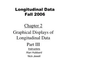
Longitudinal Data Fall 2006. Chapter 2 Graphical Displays of Longitudinal Data Part III. Instructors Alan Hubbard Nick Jewell. Outcomes vs. Explanatory Variables. Besides time, we might also be interested in the relationship of an outcome, Y ij to an explanatory variable, X ij .

E N D
Longitudinal DataFall 2006 Chapter 2 Graphical Displays of Longitudinal Data Part III Instructors Alan Hubbard Nick Jewell
Outcomes vs. Explanatory Variables • Besides time, we might also be interested in the relationship of an outcome, Yij to an explanatory variable, Xij. • The situation is relatively straightforward if examining variation in the trends in by differences in baseline covariates. • Consider examining the trends in time CD4 for groups defined by baseline viral load.
CD4 vs. time by baseline Viral Load • Perform smooth regression by Baseline Viral Load **** Plotting CD4 vs. time for strata defined by viral load ** Make categorical variable for baseline viral load gen catvl = vl500 recode catvl min/70000=0 70001/220000=1 220001/max=2 label define catvl 0 "<=70000" 1 "70001-220000" 2 ">220000" label values catvl catvl label variable catvl "Viral Load" *** Replace catvl with dummy variable if not time 0 (baseline) replace catvl = -1 if etime !=0 *** Trick to assign baseline viral load category for an id to all observations capture drop scatvl egen scatvl = max(catvl), by(id)
CD4 vs. time by baseline Viral Load, cont. ** Same program to smooth by baseline viral load gen predcd4 = . capture program drop smthbyid program define smthbyid, byable(recall) syntax [varlist] [if] [in] marksample touse capture drop predt lowess `varlist' if `touse', gen(predt) bandwidth(0.5) nograph replace predcd4 = predt if `touse' end ** Do smooths sort scatvl etime quietly by scatvl: smthbyid cd4 etime capture drop cntvl quietly by scatvl etime: gen cntvl = _n
CD4 vs. time by baseline Viral Load, cont. ** Plot gen vlow = predcd4 gen vmed = predcd4 gen vhigh = predcd4 replace vlow = . if scatvl !=0 replace vmed = . if scatvl !=1 replace vhigh = . if scatvl !=2 label variable vlow "<70000" label variable vmed "70001-220000" label variable vhigh ">220000" ** Plot #delimit ; scatter vlow etime if cntvl==1, ms(i) c(l) clpattern(solid) || scatter vmed etime if cntvl==1, ms(i) c(l) clpattern(dash) || scatter vhigh etime if cntvl==1, ms(i) c(l) clpattern(dot) ytitle("Smoothed CD4 by Basline VL") xtitle("time(days)");
Smooth regression CD4 vs. time by baseline Viral Load, cont.
Looking at longitudinal effects: Change in Y vs. Change in X(change in CD4 vs. change in viral load ) • In this case, define a new outcome variable, say Y*ij, that is the change in CD4 count from last measurement (time j-1): • Likewise, define a new explanatory variable that is the change in log10(viral load): • Use graphical techniques already discussed for CD4 versus time to this new relationship, Y*ij vs X*ij
Distribution of Viral Load and log10(viral load) – eliminating non-detects (VL <500)
Change in CD4 vs. Change in log10(viral load) ** Create X*ij, Y*ij sort id etime capture drop xdiff quietly by id: gen xdiff = logvl[_n]-logvl[_n-1] capture drop ydiff quietly by id: gen ydiff = cd4[_n]-cd4[_n-1] ** If Viral load is <=500 twice in a row, make ** observation blank by id: replace ydiff = . if vl500[_n-1]<=500 & xdiff==0 ** Smooth Y*ij vs. X*ij capture drop smthcd4vl lowess ydiff xdiff, nograph gen(smthcd4vl) ** Only want to plot smooth at unique X*ij sort xdiff capture drop cntx quietly by xdiff: gen cntx = _n
Change in CD4 vs. Change in log10(viral load) ** Plot both Smooth and Raw Data #delimit; scatter ydiff xdiff if ydiff <500 & ydiff >-500, ms(p) c(.) || scatter smthcd4vl xdiff if cntx==1, ms(i) c(l) legend(off) ytitle("Change in CD4") xtitle("Change in log10(viral load)") xlabel(-4(2)4, grid);
Just plain CD4 vs. log10(viral load)x-sectional analysis of viral load data
Summary • Raw Data Plots of Yij vs. Tij • Random sample of subjects • Evenly distributed with respect to mean, AUC, median... • Parametric (regression) models of Yij vs. Tij • Histograms of the distributions of coefficients (slopes, intercepts,...) • Raw data plotted for subjects evenly distributed with respect to coefficients • Sample of subjects fitted data, i.e., for a subset of subjects, i.
Summary • Plots of Yij vs. Tij for subjects stratified by baseline explanatory variable(s). • Change in Yij vs. change in Xij • Many more possible (e.g., surface plots of Yij vs. Xij, Tij).