Download
1 / 59
590 likes | 761 Views
Cosmological Evolution of FR II Radio Galaxies. Paramita Barai PhD Prospectus Talk Physics & Astronomy Georgia State University 19 th Oct, 2004. Contents. Introduction, Motivation, Goals & Procedures Radio Observation Samples Models of Radio Source Evolution

E N D
Cosmological Evolution of FR II Radio Galaxies Paramita Barai PhD Prospectus Talk Physics & Astronomy Georgia State University 19th Oct, 2004
Contents • Introduction, Motivation, Goals & Procedures • Radio Observation Samples • Models of Radio Source Evolution • Multi-dimensional Monte-Carlo Simulation • Results -- Fits to Observation -- Statistical Tests • Future plans P. Barai, GSU
Radio Galaxy Structure (Cygnus A) P. Barai, GSU
Fanaroff Riley Class II Radio Galaxy • The separation between the points of peak intensity in the two lobes > (½ the total size of the source). • Bright lobes & hotspot. • P > 1025 W Hz-1 sr-1 • Synchrotron radiation e-’s in the magnetic field in lobes • Unification paradigm for radio loud AGN FR II’s are parent population of radio loud QSOs (different viewing angles) P. Barai, GSU
FR Classes of Radio Galaxies P. Barai, GSU
Motivation & Wider Implications • Expansion of Radio Galaxies • Impact on galaxy formation & evolution during the quasar era (1.5 < z < 3) • From multi-frequency observations : At z~1.5 • Star & Galaxy formation rate was greater • Comoving density of radio sources – 1000 times higher • Is there a causal connection? • How much volume of the relevant universe (baryonic filaments only) do radio lobes occupy? • Could the expanding lobes trigger star formation? • Rees – 1989; De-Young – 1991; Gopal-Krishna & Wiita – 2001 P. Barai, GSU
Relevant Universe • Filaments containing baryonic material • Relevant Volume as a fraction of total Volume of Universe • 0.03 --- (z = 2: Quasar era) • 0.1 --- (z = 0) • Fig – Spatial distribution of warm / hot gas in the universe at present epoch -- Cen & Ostriker, 1999, ApJ, 514, 1 P. Barai, GSU
Observational indication of radio lobes impacting star formation: High-z RGs in Optical & Radio(Bicknell et al., 2000)
Numerical result – expanding radio lobes inducing star formation: Density contours at 0.8 Myr (left) and 1.1 Myr (right) after a RG bow shock struck a large elliptical cloud leaving dense cooling fragments (Mellema et al., 2002) P. Barai, GSU
Youth Redshift Degeneracy • Only a small fraction of actual radio galaxies at high z can be observed • Various losses as radio sources evolve • Fig from Blundell et. al., 1999 • Grey bars – luminosity range to be detectable in 7C radio galaxy survey P. Barai, GSU
Goals & Implications • Estimate: • Active life-time of radio galaxies. • The Relevant Volume Fraction of the Universe filled by Radio Lobes. • Model the Cosmological Evolution of the Radio Sources. P. Barai, GSU
Procedures • Multi-dimensional Monte-Carlo Simulation • Primordial population of radio sources generated from some early time • Redshift distribution observed Radio Luminosity Function (RLF) • Beam / Jet power distribution • Evolved by some ‘Radio Lobe Evolution Model’’ Impose survey flux limit How many detected ? • Compare w/ radio observations: • Trends in P151 (Power at 151 MHz as obs.), D (linear size), z (redshift), (spectral index) [P ~ –] • Best statistical fit Best model of Radio Galaxy Evolution P. Barai, GSU
Models • Models of evolution of radio lobes through the environment as they age: • Kaiser, Dennett-Thorpe & Alexander, 1997 (KDA) • Blundell, Rawlings & Willott, 1999 (BRW) • Manolakou & Kirk, 2002 (MK) • Best fit parameters for each model. • Sensitivity of the fits to the model parameters. • Compare these models – which is the best fit to observations? P. Barai, GSU
Observed flux dominated by the radio lobe emission Complete Sample Single flux limit P–z correlation To decouple P–z dependence use multiple complete samples at fainter flux limits Selection frequency – (Cambridge Group) – 151 & 178 MHz Least synchrotron / IC losses, orientation biases High freq. (GHz) Core contribution in flux – Doppler boosting More Synchrotron, Adiabatic & IC losses Too low freq. (<100 MHz) Losses due to: Synchrotron self-absorption Free-free absorption Low energy cut off to relativistic particles which emit via synchrotron GHz peaked sources -- not detected Frequency Selection P. Barai, GSU
Complete Observational Samples • 3CRR – • S178 > 10.9 Jy (S151 > 12.4 Jy), 4.23 sr, 145 sources. • Declination (B1950), 10 & at 10 from galactic plane • 6CE – • 2.00 S151 3.93 Jy, 0.102 sr, 58 sources. • 08h20m30s < R.A. < 13h01m30s , +3401'00" < < +4000'00" • 7CRS – (I+II+III) • S151 > 0.5 Jy, 0.022 sr, 128 sources. • 7CI – 2h < R.A. < 2.4h , 29.5° < < 34.3° • 7CII – 8.1h < R.A. < 8.4h , 24.3° < < 29.6° • 7CIII – Within 3° radius of 18h +66° P. Barai, GSU
Simplified Model of a Radio Source P. Barai, GSU
Environment Density Profile BRW & MK 0 = 1.6710–23 kg m–3 = 1.5 a0 = 10 kpc KDA 0 = 7.210–22 kg m–3 = 1.9 a0 = 2 kpc Total separation between hotspots t : Age of source Q0 : Power of each jet Radio Lobe Size Evolution P. Barai, GSU
Shared Physics in the 3 Models • Cylindrical jet moving out & accelerating particles (e–' s) at termination shock • Transport of relativistic particles (e– 's) from head to lobe -- emitting (in radio) via Synchrotron mechanism • Power Losses: • Adiabatic loss (as source expands) • Inverse Compton scattering off CMB photons • Synchrotron radiation • Intricacies of the models are different P. Barai, GSU
e– 's initially accelerated First–order Fermi process at termination shock Energy distribution is power-law function of initial Lorentz factor Injection index: p = 2.14 uCMB ~ (z+1)4 Taken Constant for a source born at z Cocoon (lobe): pc ~ t(–4–)/(5–) : density exponent in external atmosphere ph / pc ~ 4RT2 RT = Axial Ratio = Length / Width = 2 5 RT 1.3 Key Assumptions of KDA Model P. Barai, GSU
phead/plobe = 6 Injection index (p) governed by break frequencies Main diff. from KDA Break in frequency spectrum of synchrotron emission break in energy spectrum of freshly injected particles Longest & shortest times particles are lingering in hotspot before injection into lobe -- Slow & Fast Break Frequencies -- bs & bf BRW Lobe Luminosity P. Barai, GSU
Adiabatic losses in head compensated (by some turbulent re-acceleration process) during transport b/w jet termination shock & lobe Parameter describes the transport = 1 --- Diffusion Range of escape times for particles from high-loss head region MK Power Evolution P. Barai, GSU
tbir , tage , (zobs), Q0 For each source Sources born every 106 years – from z = 10 tbir tmax-age = 500 Myr Relevant Comoving Volume Volume of shell where source must be present s.t. we see it today w/in a max age of 500 MYr R(t) – Scale factor of Universe = r (FLAT space time) Generating Primordial Radio Source Population P. Barai, GSU
Redshift distribution # per unit comov. vol: z0 = 2.2 z0 = 0.6 V (z) # of Sources Sources allocated radial coord. () -- uniform distribution within comoving volume tage = tobs - tbir Initial Power distribution if, Qmin < Q0 < Qmax Qmin = 51037 W Qmax = 51042 W x = 2.6 Multi-Dimensional Monte-Carlo Simulation P. Barai, GSU
Radio Luminosity Function (Willott et. al. 2001) • Willott et. al. P. Barai, GSU
Newest RLF Grimes et. al., 2004 (GRW) z2a = 1.684 z2b = 0.447 RLF from GRW P. Barai, GSU
Some plot showing the sources generated (a small sample) ?? • Tage vs. z • Q vs z • Tbir vs. z P. Barai, GSU
Fraction of Relevant Universe filled by Radio Lobes (Alternative model) • Cosmological evolution of the ambient gas density • Case 1: Power law ambient density • Case 2: Constant density medium: • Total mass contained within a sphere of R Mpc = N Mass within the standard z = 0 extended halo. • For z = 2.5, N = 30 is reasonable (since relevant volume fraction = 0.10 and about 50 % of the mass is in the filaments at z = 0). P. Barai, GSU
Volumes filled by Radio Lobes over time, for the power-law model (Case 1: V1) & the dense IGM model (Case 2: V2, N=30, R=5Mpc).
Kolmogorov – Smirnov (K–S) statistics to test fits of the 3 models : P(K–S)Fractional Probability that the quantities of model prediction and observation are drawn from same cumulative distribution population