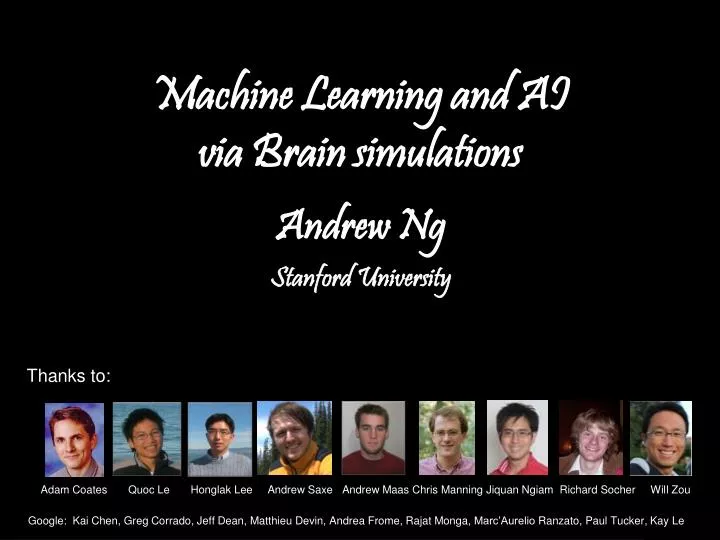
Machine Learning and AI via Brain simulations

1. Machine Learning and AI via Brain simulations Andrew Ng Stanford University Thanks to: Adam Coates Quoc Le Honglak Lee Andrew Saxe Andrew Maas Chris Manning Jiquan Ngiam Richard Socher Will Zou Google: Kai Chen, Greg Corrado, Jeff Dean, Matthieu Devin, Andrea Frome, RajatMonga, Marc’AurelioRanzato, Paul Tucker, Kay Le

2. This talk: Deep Learning Using brain simulations: - Make learning algorithms much better and easier to use. - Make revolutionary advances in machine learning and AI. Vision shared with many researchers: E.g., Samy Bengio, Yoshua Bengio, Tom Dean, Jeff Dean, Nando de Freitas, Jeff Hawkins, Geoff Hinton, Quoc Le, Yann LeCun, Honglak Lee, Tommy Poggio, Marc’AurelioRanzato, RuslanSalakhutdinov, Josh Tenenbaum, Kai Yu, Jason Weston, …. I believe this is our best shot at progress towards real AI.

3. What do we want computers to do with our data? Label: “Motorcycle” Suggest tags Image search … Images/video Audio Text Speech recognition Music classification Speaker identification … Web search Anti-spam Machine translation …

4. Computer vision is hard! Motorcycle Motorcycle Motorcycle Motorcycle Motorcycle Motorcycle Motorcycle Motorcycle Motorcycle

5. What do we want computers to do with our data? Label: “Motorcycle” Suggest tags Image search … Images/video Audio Text Speech recognition Speaker identification Music classification … Web search Anti-spam Machine translation … Machine learning performs well on many of these problems, but is a lot of work. What is it about machine learning that makes it so hard to use?

6. Machine learning for image classification “Motorcycle” This talk: Develop ideas using images and audio. Ideas apply to other problems (e.g., text) too.

7. But the camera sees this: Why is this hard? You see this:

8. Machine learning and feature representations pixel 1 Learning algorithm pixel 2 Input Motorbikes “Non”-Motorbikes Raw image pixel 2 pixel 1

9. Machine learning and feature representations pixel 1 Learning algorithm pixel 2 Input Motorbikes “Non”-Motorbikes Raw image pixel 2 pixel 1

10. Machine learning and feature representations pixel 1 Learning algorithm pixel 2 Input Motorbikes “Non”-Motorbikes Raw image pixel 2 pixel 1

11. What we want handlebars Feature representation Learning algorithm wheel Input E.g., Does it have Handlebars? Wheels? Motorbikes “Non”-Motorbikes Raw image Features pixel 2 Wheels pixel 1 Handlebars

12. How is computer perception done? Images/video Detection Vision features Image Audio Audio Audio features Speaker ID Text classification, Machine translation, Information retrieval, .... Image Grasp point Low-level features Text Text features Text

13. Feature representations Learning algorithm Feature Representation Input

14. Computer vision features SIFT Spin image HoG RIFT GLOH Textons

15. Audio features MFCC Spectrogram Flux Rolloff ZCR

16. NLP features Named entity recognition Stemming Parser features Coming up with features is difficult, time-consuming, requires expert knowledge. “Applied machine learning” is basically feature engineering. Part of speech Anaphora Ontologies (WordNet)

17. Feature representations Learning algorithm Feature Representation Input

18. The “one learning algorithm” hypothesis Auditory Cortex Auditory cortex learns to see [Roe et al., 1992]

19. The “one learning algorithm” hypothesis Somatosensory Cortex Somatosensory cortex learns to see [Metin & Frost, 1989]

20. Sensor representations in the brain Seeing with your tongue Human echolocation (sonar) Implanting a 3rd eye Haptic belt: Direction sense [BrainPort; Welsh & Blasch, 1997; Nagel et al., 2005; Constantine-Paton & Law, 2009]

21. Feature learning problem • Given a 14x14 image patch x, can represent it using 196 real numbers. • Problem: Can we find a learn a better feature vector to represent this? 255 98 93 87 89 91 48 …

22. First stage of visual processing: V1 V1 is the first stage of visual processing in the brain. Neurons in V1 typically modeled as edge detectors: Neuron #1 of visual cortex (model) Neuron #2 of visual cortex (model)

23. Learning sensor representations Sparse coding (Olshausen & Field,1996) Input: Images x(1), x(2), …, x(m)(each in Rn x n) Learn: Dictionary of bases f1, f2, …, fk(also Rn x n), so that each input x can be approximately decomposed as: xajfj s.t. aj’s are mostly zero (“sparse”) Use to represent 14x14 image patch succinctly, as [a7=0.8, a36=0.3, a41 = 0.5]. I.e., this indicates which “basic edges” make up the image. k j=1 [NIPS 2006, 2007]

24. Sparse coding illustration Natural Images Learned bases (f1 , …, f64): “Edges” »0.8 * + 0.3 * + 0.5 * Test example x»0.8 * f36+ 0.3 * f42+ 0.5 * f63 [a1, …, a64] = [0, 0, …, 0,0.8, 0, …, 0, 0.3, 0, …, 0, 0.5, 0] (feature representation) More succinct, higher-level, representation.

25. 0.6 *+ 0.8 *+ 0.4 * 15 28 37 1.3 *+ 0.9 *+ 0.3 * 5 18 29 More examples Represent as: [a15=0.6, a28=0.8, a37 = 0.4]. Represent as: [a5=1.3, a18=0.9, a29 = 0.3]. • Method “invents” edge detection. • Automatically learns to represent an image in terms of the edges that appear in it. Gives a more succinct, higher-level representation than the raw pixels. • Quantitatively similar to primary visual cortex (area V1) in brain.

26. Sparse coding applied to audio Image shows 20 basis functions learned from unlabeled audio. [Evan Smith & Mike Lewicki, 2006]

27. Sparse coding applied to audio Image shows 20 basis functions learned from unlabeled audio. [Evan Smith & Mike Lewicki, 2006]

28. Learning feature hierarchies Higher layer (Combinations of edges; cf. V2) a1 a2 a3 “Sparse coding” (edges; cf. V1) x1 x2 x3 x4 Input image (pixels) [Technical details: Sparse autoencoder or sparse version of Hinton’s DBN.] [Lee, Ranganath & Ng, 2007]

29. Learning feature hierarchies Higher layer (Model V3?) Higher layer (Model V2?) a1 a2 a3 Model V1 x1 x2 x3 x4 Input image [Technical details: Sparse autoencoder or sparse version of Hinton’s DBN.] [Lee, Ranganath & Ng, 2007]

30. Hierarchical Sparse coding (Sparse DBN): Trained on face images object models object parts (combination of edges) Training set: Aligned images of faces. edges pixels [Honglak Lee]

31. Machine learning applications

32. Unsupervised feature learning (Self-taught learning) Motorcycles Not motorcycles Testing: What is this? … Unlabeled images [Lee, Raina and Ng, 2006; Raina, Lee, Battle, Packer & Ng, 2007] [This uses unlabeled data. One can learn the features from labeled data too.]

33. Video Activity recognition (Hollywood 2 benchmark) Unsupervised feature learning significantly improves on the previous state-of-the-art. [Le, Zhou & Ng, 2011]

34. Audio Images Galaxy Video Text/NLP Multimodal (audio/video)

35. How do you build a high accuracy learning system?

36. Supervised Learning: Labeled data • Choices of learning algorithm: • Memory based • Winnow • Perceptron • Naïve Bayes • SVM • …. • What matters the most? Accuracy Training set size (millions) [Banko & Brill, 2001] “It’s not who has the best algorithm that wins. It’s who has the most data.”

37. Unsupervised Learning Large numbers of features is critical. The specific learning algorithm is important, but ones that can scale to many features also have a big advantage. [Adam Coates]

39. Learning from Labeled data

40. Training Data Model

41. Machine (Model Partition) Training Data Model

42. Core Machine (Model Partition) Training Data Model

43. Unsupervised or Supervised Objective Minibatch Stochastic Gradient Descent (SGD) Model parameters sharded by partition 10s, 100s, or 1000s of cores per model Training Data Basic DistBelief Model Training Model

44. Training Data Basic DistBelief Model Training Model Parallelize across ~100 machines (~1600 cores). But training is still slow with large data sets. Add another dimension of parallelism, and have multiple model instances in parallel.

45. ∆p ∆p’ p’ p Asynchronous Distributed Stochastic Gradient Descent p’ = p + ∆p p’’ = p’ + ∆p’ Parameter Server Model Data

46. Asynchronous Distributed Stochastic Gradient Descent p’ = p + ∆p Parameter Server ∆p p’ Model Workers Data Shards

47. Better robustness to individual slow machines Makes forward progress even during evictions/restarts Parameter Server Slavemodels Data Shards Asynchronous Distributed Stochastic Gradient Descent From an engineering standpoint, superior to a single model with the same number of total machines:

48. Acoustic Modeling for Speech Recognition Async SGD and L-BFGS can both speed up model training. To reach the same model quality DistBeliefreached in 4 days took 55 days using a GPU.... DistBelief can support much larger models than a GPU (useful for unsupervised learning).

50. Speech recognition on Android